The following parameters updates correspond to the upcoming paper: Impact of an Early BMI Maintenance Intervention at ART initiation on Diabetes Risk: Insights from a Simulation Study
Parametrization
PEARL simulations begin in 2009 by creating an initial population of HIV-infected individuals, either receiving ART or disengaged from care in the US (Figure 1). The population size and the distribution of their ages, ART initiation years, and CD4 counts at initiation are estimated using data from NA-ACCORD and the CDC. At the start of each simulated year (2010–2030), a population of new ART initiators enter the model. The population size, age, and CD4 count distributions at ART initiation are derived from CDC and NA-ACCORD data. Individuals on ART face a risk of mortality and disengagement from care over time. Upon disengagement, the probability of mortality increases, and CD4 counts gradually decline. The CD4 count for all individuals is updated over time depending on their HIV care status—rising for those in care and declining for those out of care.
Additionally, PEARL simulates a range of mental and physical comorbidities among individuals aging with HIV. These comorbid conditions are divided into multiple stages based on their modeling in the simulation. Smoking, BMI, and hepatitis C virus are considered risk factors; anxiety and depression are classified as stage 1; chronic kidney disease, hyperlipidemia, diabetes mellitus, and hypertension are stage 2; and cancer, end-stage liver disease, and myocardial infarction are stage 3. The incidence of conditions in a given stage is influenced by the presence of conditions from prior stages as well as other factors, as outlined below. Mortality functions are also adjusted to account for the presence of comorbidities.
All comorbidity parameters are derived from the NA-ACCORD data between 2009-2017. Simulated outcomes, such as the age distribution of the population in HIV care and the incidence and prevalence of comorbidities, are cross-validated with NA-ACCORD data from this period[1, 2]. Model projections extend from 2018 to 2030.
In this section, we provide a brief discussion of key parameters related to the population starting ART, BMI dynamics, and the risk of diabetes in the model. This discussion aims to clarify the key assumptions used to parametrize these factors and their potential role in shaping the projected outcomes.
Population Initiating ART From 2010 - 2030
Population Size
New HIV diagnosis: In order to predict the number of new people linking to HIV care and starting ART in a given year, we begin with data on the number of new HIV diagnoses per year as estimated by the CDC’s Medical Monitoring Project (MMP) as shown in Table 6. Dates before 2016 came from Table 1 of the 2015 HIV Surveillance Report, while data 2016 and after came from Table 1 of the 2018 HIV Surveillance Report.
Table 6: Number of New HIV Diagnoses by Year
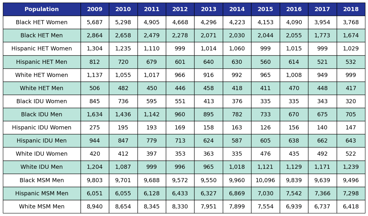
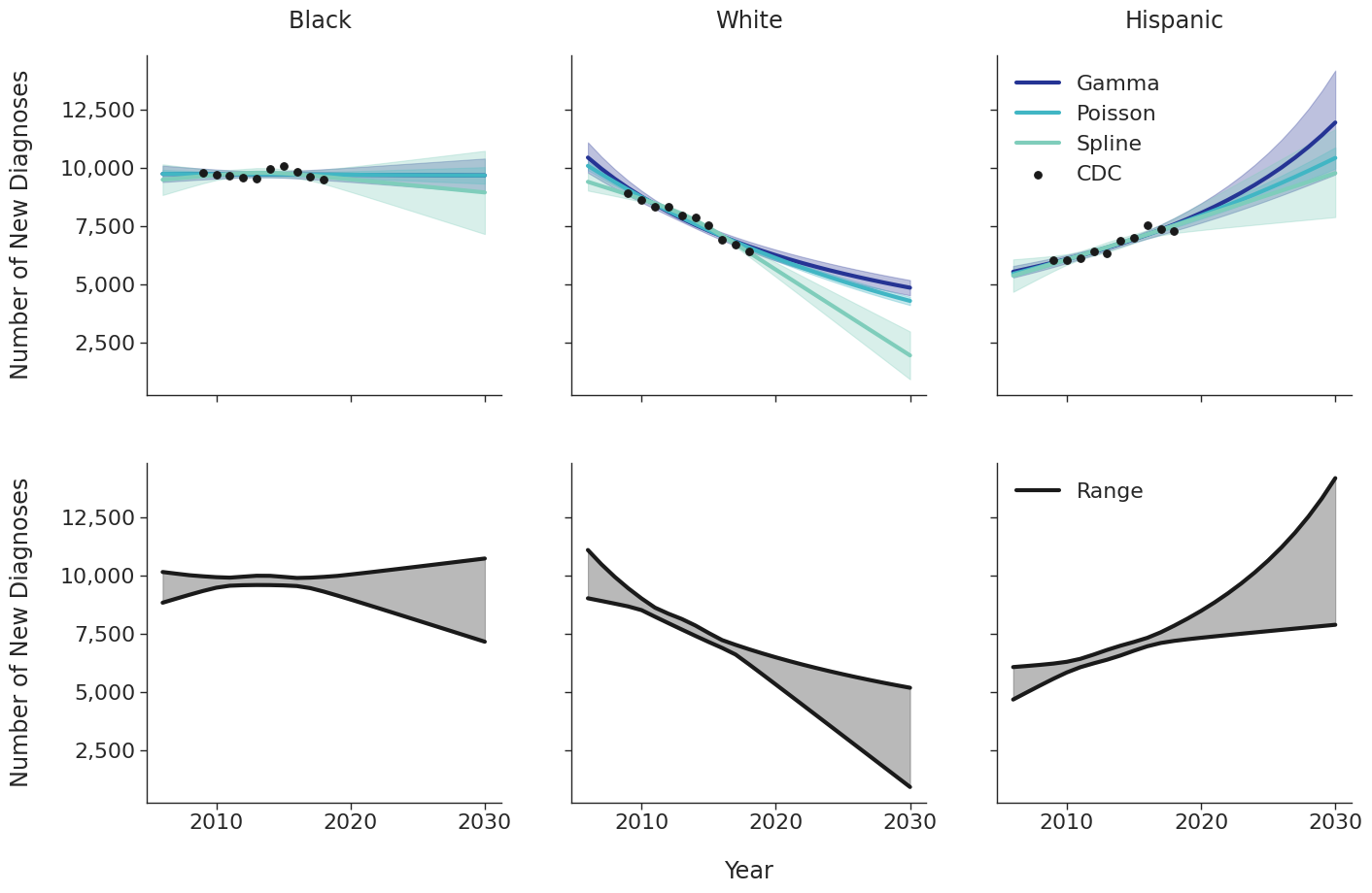
Various candidate models were proposed in order to predict the number of new HIV diagnoses from 2006 to 2030. Predicted HIV diagnoses prior to 2010 are used later in the initial 2009 population creation. After removing models with inadequate fit (based on AIC values), the data were fit using a Poisson model, a gamma model and a natural cubic spline model with a single knot. Of these models, those resulting in unrealistic projections (>50% increase in new diagnosis from 2020 – 2030) were also removed. The Poisson and gamma fits were accomplished using the glm function of the stats package in base R, while the spline fit was generated using the lm and ns functions of the base R packages stats and splines, respectively. To incorporate additional uncertainties in annual estimates, the 95% prediction intervals around each fit were calculated. These prediction intervals were combined to generate an annual range for the number of new diagnosis in each year for a given subgroup (black, white and Hispanic). The annual ranges are estimated from the largest upper prediction interval and the lowest lower prediction interval of existing models as shown in panel 2 of Figure 3. For each simulation run, a random number between 0 and 1 is drawn that defines the number of new diagnoses in that simulation. Figure 3 shows the full ranges used to generate the number of new diagnoses.
Figure 3a: HET Female
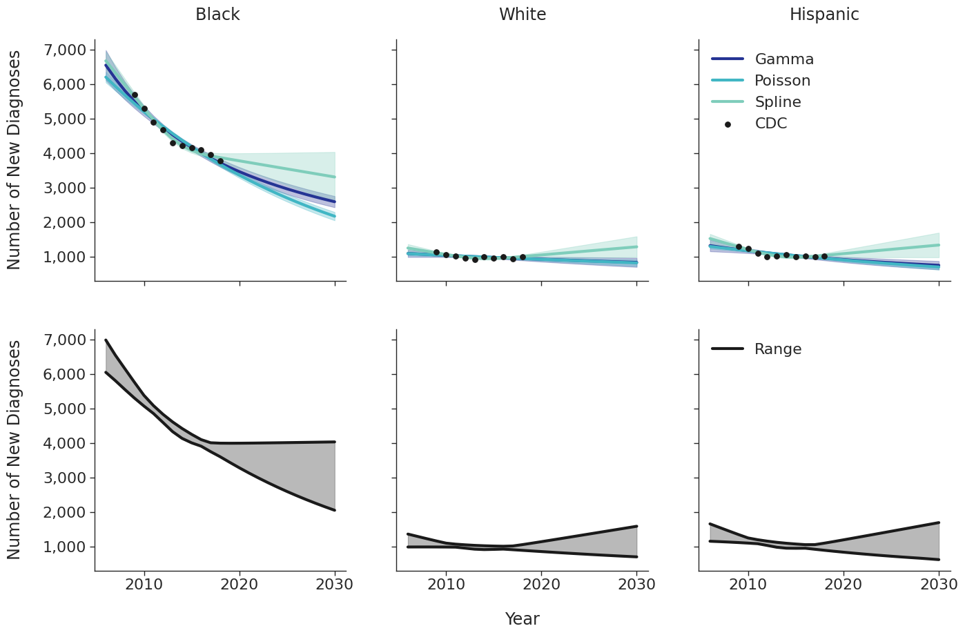
Figure 3b: HET Male
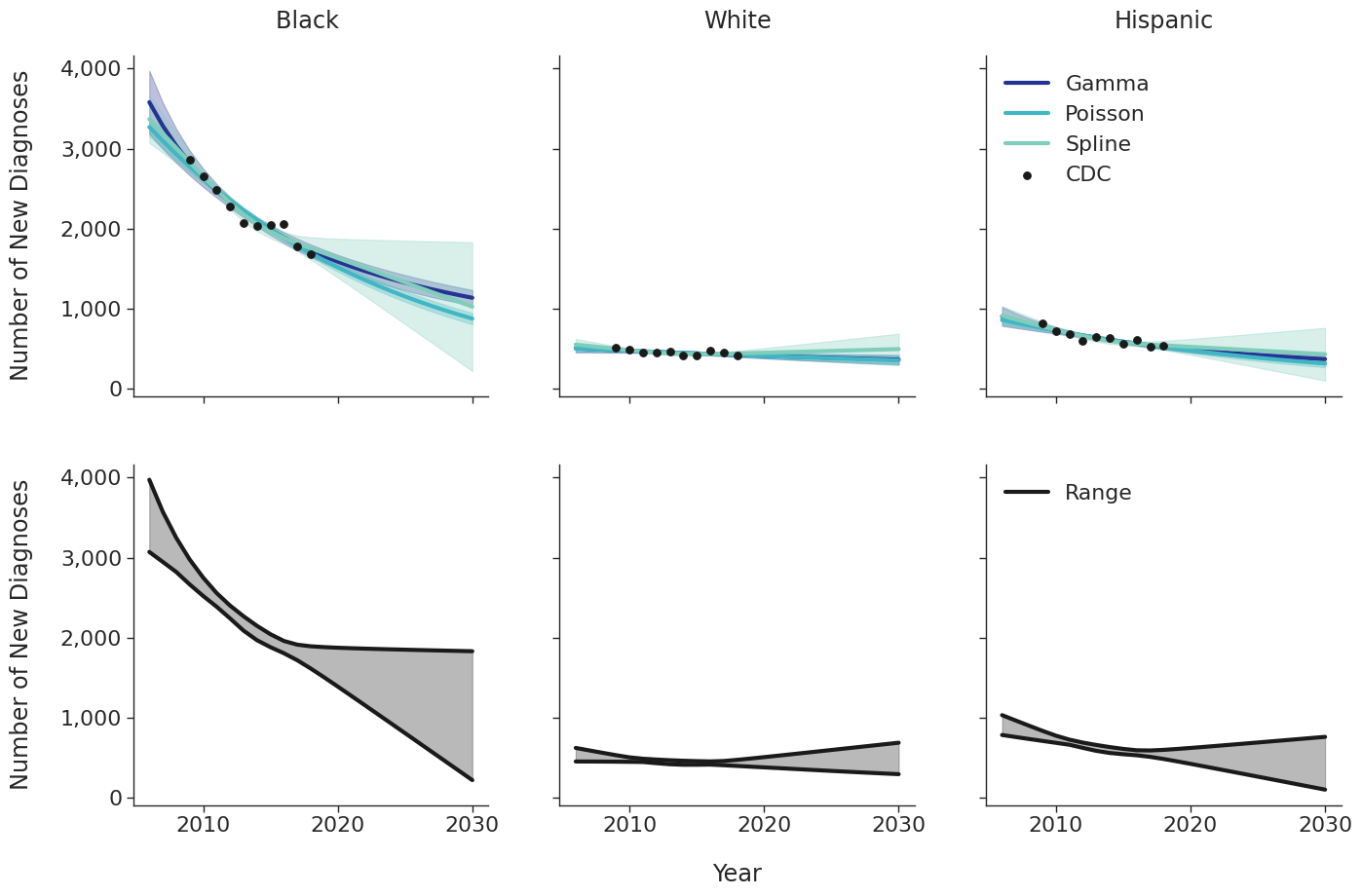
Figure 3c: IDU Female
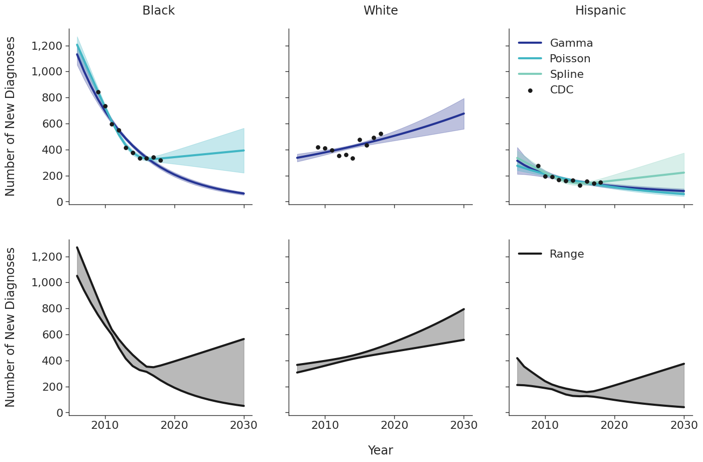
Figure 3d: IDU Male
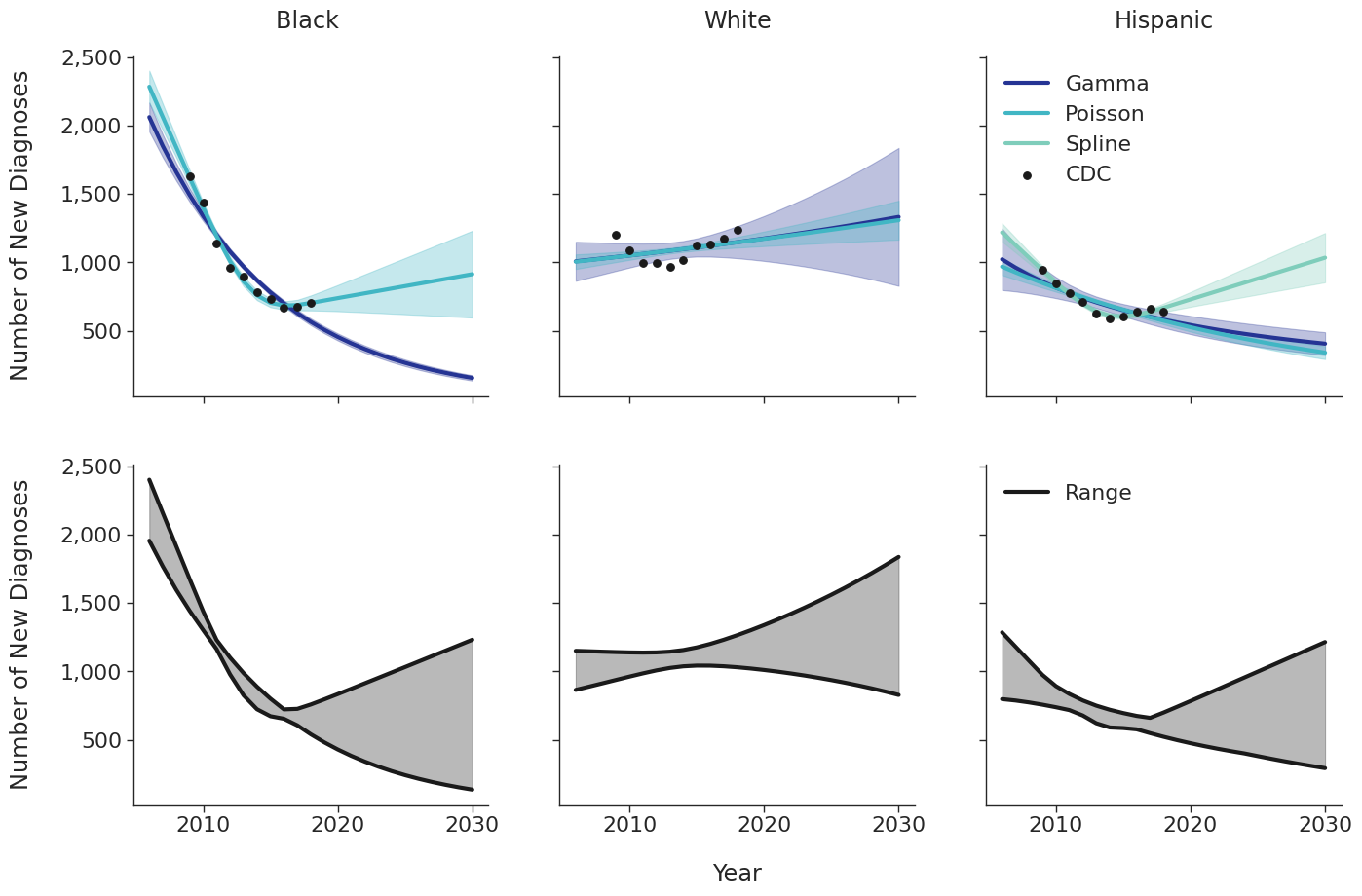
Figure 3e: MSM
Modeling BMI Dynamics in PEARL
Body Mass Index (BMI) measurements are analyzed in relation to the initiation of ART. BMI data from NA-ACCORD are categorized into pre-ART and post-ART windows for comparison and analysis. Pre-ART BMI is defined as any BMI measurement taken in the window starting 365 days prior to ART initiation and extending to 90 days after ART initiation. If multiple BMI measurements are recorded within this window, the median value is used to minimize the impact of measurement errors or outliers. Post-ART BMI is defined as any BMI measurement taken in the period starting 365 days after ART initiation and extending to 730 days (365 × 2) after ART initiation. As with the pre-ART BMI, if more than one measurement is recorded within this window, the median is taken for representing post-ART BMI. If a patient’s ART initiation date falls outside of their cohort’s BMI observation window, BMI values (both pre-ART and post-ART) are not calculated for that patient to ensure data consistency. In addition to BMI, the median CD4 count in the post-ART window (365 days to 730 days after ART initiation) is calculated for each patient. This will later be used as a variable in regression models predicting post-ART BMI, contributing to the understanding of the relationship between immune status and BMI changes following ART initiation.
Pre-ART BMI
Pre-ART BMI (pre_art_bmi) is modeling log_10〖pre_art_bmi〗 as linear functions of 6 different combinations from age, age category, restricted cubic splines of age, year of ART initiation and restricted cubic spline of year of ART initiation (Table S1). To identify the best-fitting model for each analysis, the Akaike Information Criterion (AIC) is used as a selection criterion (Table S2). AIC is a widely used measure for comparing the goodness of fit among multiple statistical models while penalizing for model complexity. It balances the trade-off between the model’s fit and the number of parameters used, helping to avoid overfitting. Four final models are determined for different subpopulations to capture the important clinical effect of change in BMI resulting from ART treatment.
Table: Total ART Users in 2009
| Model List | Age Input Type | Year of ART Initiation Input Type |
|---|---|---|
| Candidate Model 1 | Categorical | Continuous Variable |
| Candidate Model 2 | Categorical | Restricted Cubic Spline |
| Candidate Model 3 | Continuous Variable | Continuous Variable |
| Candidate Model 4 | Restricted Cubic Spline | Restricted Cubic Spline |
| Candidate Model 5 | Restricted Cubic Spline | Continuous Variable |
| Candidate Model 6 | Restricted Cubic Spline | Restricted Cubic Spline |
Table: Pre-ART BMI Candidate Model AIC
| Race/Risk | Sex | Model 1 AIC | Model 2 AIC | Model 3 AIC | Model 4 AIC | Model 5 AIC | Model 6 AIC | Smallest AIC value | Final Model |
|---|---|---|---|---|---|---|---|---|---|
| HET Black/AA | Female | -4517.1 | -4515.6 | -4520.8 | -4519.4 | -4522.3 | -4520.8 | -4522.3 | Model 5 |
| HET Hispanic | Female | -851.59 | -853.3 | -851.59 | -853.59 | -854.47 | -855.88 | -855.88 | Model 3 |
| HET White | Female | -1025.1 | -1021.6 | -1028.6 | -1025.2 | -1024.7 | -1021.3 | -1028.6 | Model 3 |
| IDU Black/AA | Female | -632.61 | -628.77 | -638.13 | -634.37 | -634.54 | -630.73 | -638.13 | Model 3 |
| IDU Hispanic White | Female | -505.18 | -502.7 | -511.6 | -509.25 | -509.25 | -507.2 | -511.6 | Model 3 |
| HET Black | Male | -4054.2 | -4053 | -4039 | -4038.4 | -4056.7 | -4055.8 | -4056.7 | Model 5 |
| HET Hispanic | Male | -1364.4 | -1362.4 | -1368.5 | -1366.4 | -1369 | -1366.8 | -1369 | Model 5 |
| HET White | Male | -1257.5 | -1255.3 | -1262.8 | -1260.6 | -1259.3 | -1257 | -1262.8 | Model 3 |
| IDU Black/AA | Male | -6479.4 | -6478.3 | -6461.5 | -6461 | -6484.2 | -6482.8 | -6484.2 | Model 5 |
| IDU Hispanic | Male | -1125.3 | -1126.2 | -1119.6 | -1120.1 | -1122.1 | -1123.3 | -1126.2 | Model 2 |
| IDU White | Male | -4496 | -4498.2 | -4494.3 | -4496.6 | -4498.5 | -4500.6 | -4500.6 | Model 6 |
| MSM Black/AA | Male | -8293.1 | -8289.1 | -8266.4 | -8262.6 | -8323 | -8319.2 | -8323 | Model 5 |
| MSM Hispanic | Male | -5341.4 | -5340.1 | -5340.1 | -5339.4 | -5348.6 | -5347.5 | -5348.6 | Model 5 |
| MSM White | Male | -15172 | -15171 | -15091 | -15090 | -15213 | -15212 | -15213 | Model 5 |
Model 1
Model 1 is used only by the \(\mathrm{idu\_hisp\_male}\) population. We model \(\log_{10}(\mathrm{pre\_art\_bmi})\) as a function of age category (\(\mathrm{age\_cat}\)) and \(\mathrm{art\_init\_year}\). The age categories are given by
\[\mathrm{age\_cat\_1\ =\ }\left\{\begin{matrix}1,&30\le\ \mathrm{age\ \le\ \ } 39\mathrm{\ } \\0,&\mathrm{else},\\\end{matrix}\right.\] \[\mathrm{age\_cat\_2\ =\ }\left\{\begin{matrix}1,&40\le\ \mathrm{age\ \le\ \ } 49\mathrm{\ } \\0,&\mathrm{else},\\\end{matrix}\right.\] \[\mathrm{age\_cat\_3\ =\ }\left\{\begin{matrix}1,&50\le\ \mathrm{age\ \le\ \ } 59\mathrm{\ } \\0,&\mathrm{else},\\\end{matrix}\right.\]and
\[\mathrm{age\_cat\_4\ =\ }\left\{\begin{matrix}1,&60\le\ \mathrm{age\ \ } \\0,&\mathrm{else}.\\\end{matrix}\right.\]A restricted cubic spline is used to model \(\mathrm{art\_init\_year}\) with the following knots:
Table 19: Pre-ART BMI Model 1 Knots

The full function is given by:
\[\begin{split} \log_{10}(\mathrm{pre\_art\_bmi}) = \beta_0 &+ \beta_\mathrm{age\_cat\_1} \cdot \mathrm{age\_cat\_1} + \beta_\mathrm{age\_cat\_2} \cdot \mathrm{age\_cat\_2} + \beta_\mathrm{age\_cat\_3} \cdot \mathrm{age\_cat\_3} + \beta_\mathrm{age\_cat\_4} \cdot \mathrm{age\_cat\_4}\\[2ex] &+ \beta_\mathrm{art\_init\_year} \cdot \mathrm{art\_init\_year}+ \beta_\mathrm{art\_init\_year\_1} \cdot \mathrm{art\_init\_year\_1} + \beta_\mathrm{art\_init\_year\_2} \cdot \mathrm{art\_init\_year\_2} \end{split}\]Table 20: Pre-ART BMI Model 1 Estimates

Model 2
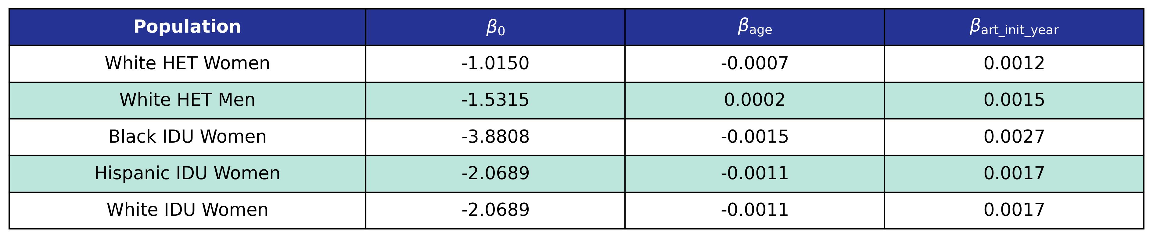
Model 2 is used by the \(\mathrm{het\_white\_female}\), \(\mathrm{het\_white\_male}\), \(\mathrm{idu\_black\_female}\), \(\mathrm{idu\_hisp\_female}\), and \(\mathrm{idu\_white\_female}\) populations. We model \(\log_{10}(\mathrm{pre\_art\_bmi})\) as a linear function of \(\mathrm{age}\) and \(\mathrm{art\_init\_year}\)
\[\log_{10}(\mathrm{pre\_art\_bmi}) = \beta_0 + \beta_\mathrm{age} \cdot \mathrm{age} + \beta_\mathrm{art\_init\_year} \cdot \mathrm{art\_init\_year}\]Table 21: Pre-ART BMI Model 2 Estimates
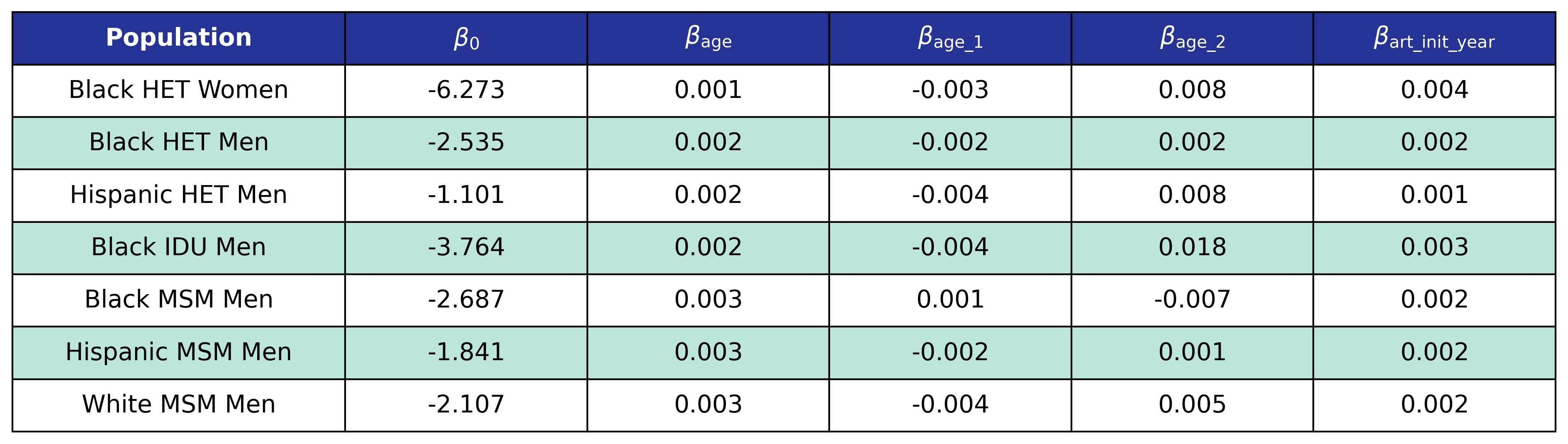
Model 3
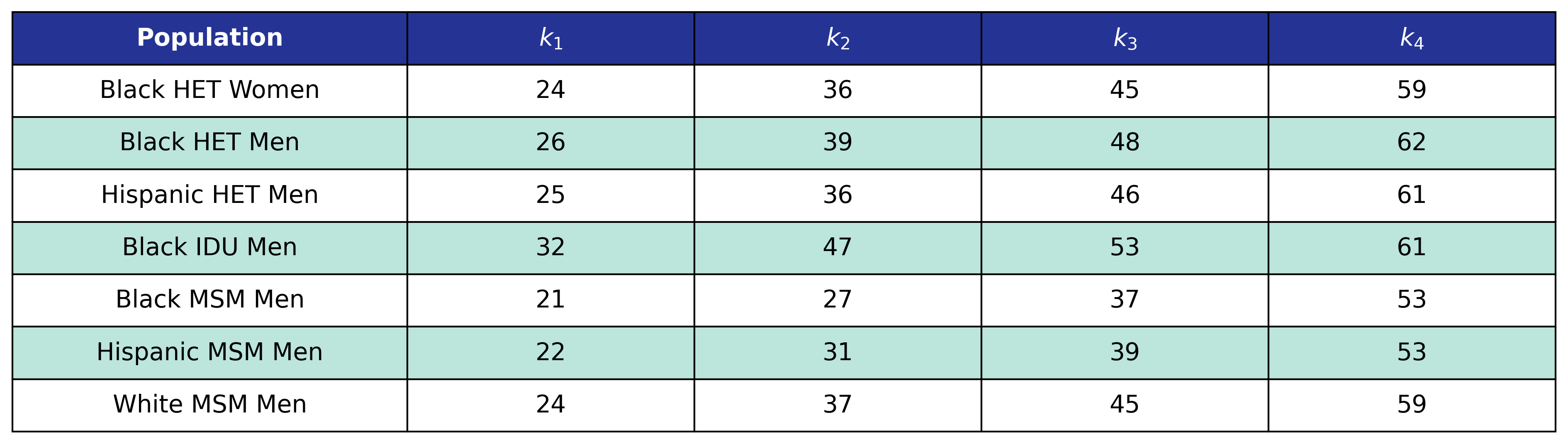
Model 3 is used by the \(\mathrm{het\_black\_female}\), \(\mathrm{het\_black\_male}\), \(\mathrm{het\_hisp\_male}\), \(\mathrm{idu\_black\_male}\), \(\mathrm{msm\_black\_male}\), \(\mathrm{msm\_hisp\_male}\), and \(\mathrm{msm\_white\_male}\) populations. We model \(\log_{10}(\mathrm{pre\_art\_bmi})\) as a restricted cubic spline function of \(\mathrm{age}\) and a linear function of \(\mathrm{art\_init\_year}\).
Table 22: Pre-ART BMI Model 3 Knots
The function and its estimates follow.
\[\log_{10}(\mathrm{pre\_art\_bmi}) = \beta_0 + \beta_\mathrm{age} \cdot \mathrm{age} + \beta_\mathrm{age\_1} \cdot \mathrm{age\_1} + \beta_\mathrm{age\_2} \cdot \mathrm{age\_2} + \beta_\mathrm{art\_init\_year} \cdot \mathrm{art\_init\_year}\]Table 23: Pre-ART BMI Model 3 Estimates
Model 4
Model 2 is used by the \(\mathrm{het\_hisp\_female}\) and \(\mathrm{idu\_white\_male}\) populations. We model \(\log_{10}(\mathrm{pre\_art\_bmi})\) as a restricted cubic spline function of age \(\mathrm{age}\) and \(\mathrm{art\_init\_year}\).
Table 24: Pre-ART BMI Model 4 Age Knots

Table 25: Pre-ART BMI Model 4 ART Initiation Year Knots

The function and its estimates are:
\[\begin{split} \log_{10}(\mathrm{pre\_art\_bmi}) = \beta_0 &+ \beta_\mathrm{age} \cdot \mathrm{age} + \beta_\mathrm{age\_1} \cdot \mathrm{age\_1} + \beta_\mathrm{age\_2} \cdot \mathrm{age\_2}+ \beta_\mathrm{art\_init\_year} \cdot \mathrm{art\_init\_year}\\[2ex] &+ \beta_\mathrm{art\_init\_year\_1} \cdot \mathrm{art\_init\_year\_1} + \beta_\mathrm{art\_init\_year\_2} \cdot \mathrm{art\_init\_year\_2} \end{split}\]Table 26: Pre-ART BMI Model 4 Estimates

Post-ART BMI
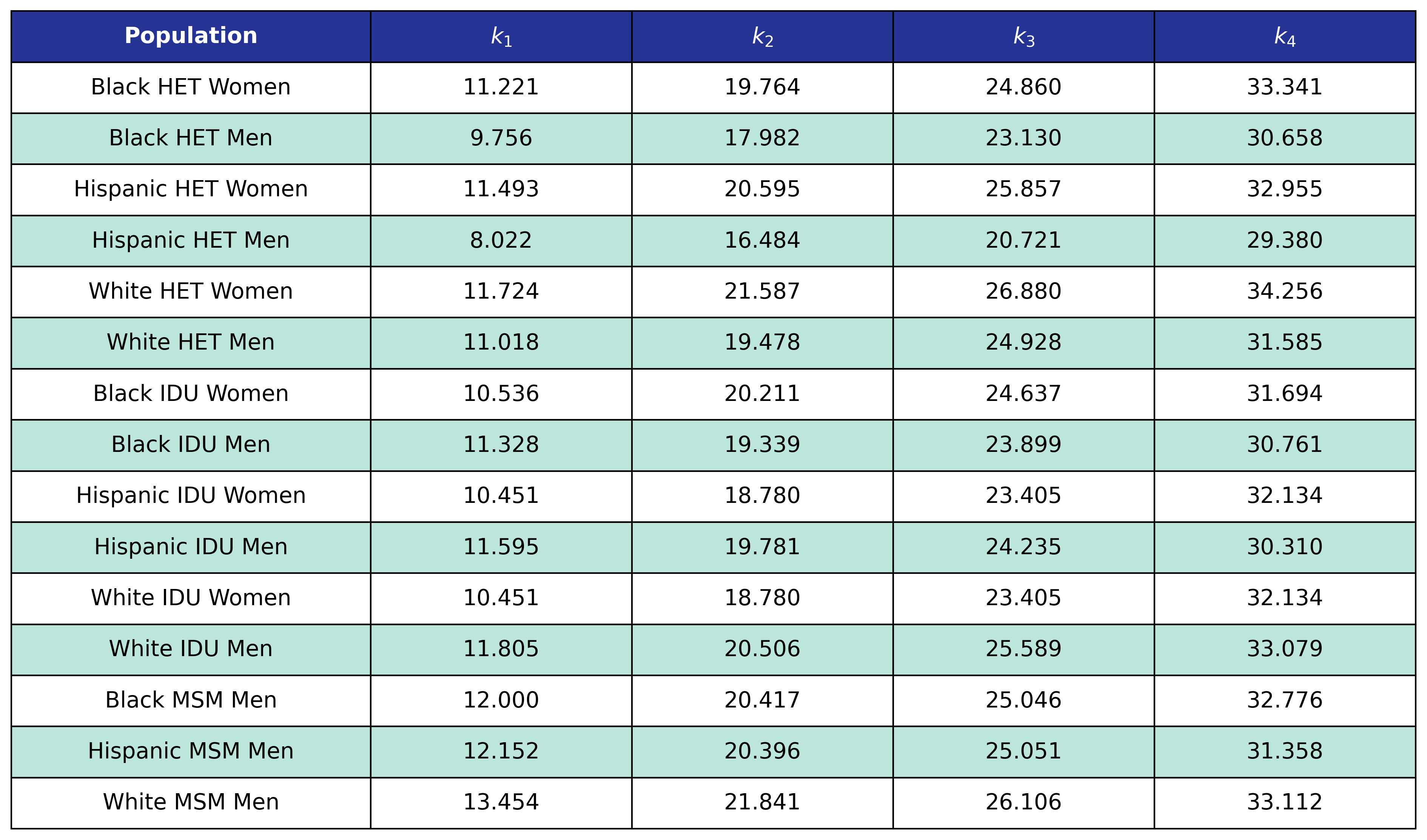
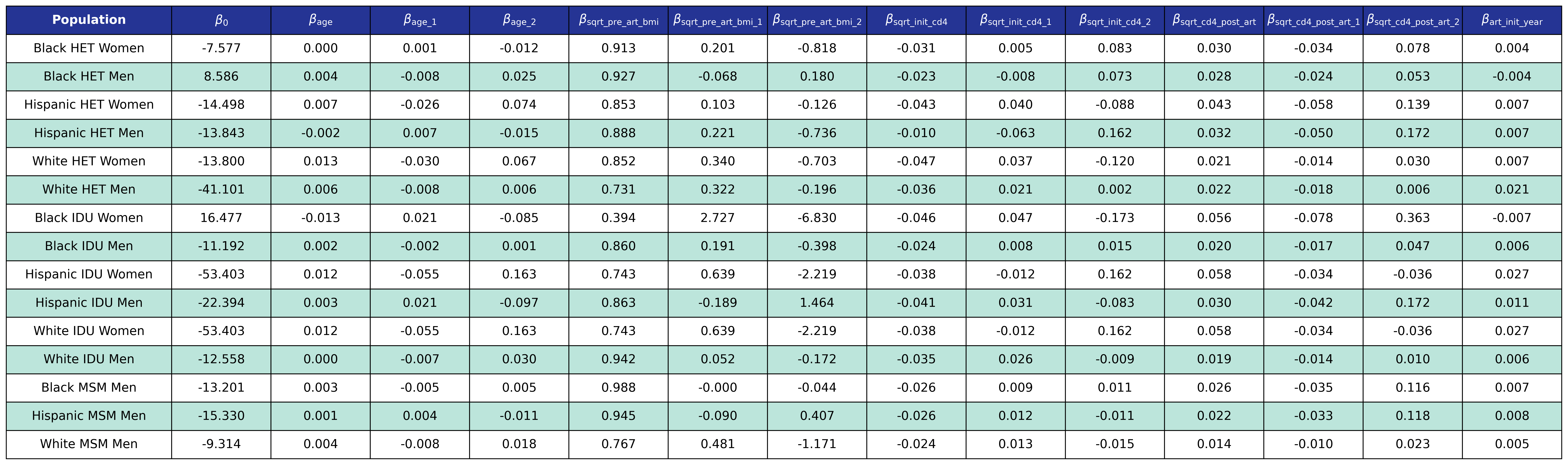
Post-ART BMI (\(\mathrm{post\_art\_bmi}\)) is calculated using only a single model for all 15 subpopulations. We model \(\mathrm{sqrt\_post\_art\_bmi}\) as a function of \(\mathrm{age}\), square root of pre-ART BMI (\(\mathrm{sqrt\_pre\_art\_bmi}\)), square root of CD4 count at ART initiation (\(\mathrm{sqrt\_init\_cd4}\)), and square root of CD4 count 2 years after ART initiation (\(\mathrm{sqrt\_cd4\_post\_art}\)) modeled by restricted cubic splines as well as a linear function of \(\mathrm{art\_init\_year}\). The full equation is:
\[\begin{split} \mathrm{sqrt\_post\_art\_bmi} = \beta_0 &+ \beta_\mathrm{age} \cdot \mathrm{age} + \beta_\mathrm{age\_1} \cdot \mathrm{age\_1} + \beta_\mathrm{age\_2} \cdot \mathrm{age\_2} + \beta_\mathrm{sqrt\_pre\_art\_bmi} \cdot \mathrm{sqrt\_pre\_art\_bmi}\\[2ex] &+ \beta_\mathrm{sqrt\_pre\_art\_bmi\_1} \cdot \mathrm{sqrt\_pre\_art\_bmi\_1}+ \beta_\mathrm{sqrt\_pre\_art\_bmi\_2} \cdot \mathrm{sqrt\_pre\_art\_bmi\_2}\\[2ex] &+ \beta_\mathrm{sqrt\_init\_cd4} \cdot \mathrm{sqrt\_init\_cd4} + \beta_\mathrm{sqrt\_init\_cd4\_1} \cdot \mathrm{sqrt\_init\_cd4\_1} + \beta_\mathrm{sqrt\_init\_cd4\_2} \cdot \mathrm{sqrt\_init\_cd4\_2}\\[2ex] &+ \beta_\mathrm{sqrt\_cd4\_post\_art} \cdot \mathrm{sqrt\_cd4\_post\_art} + \beta_\mathrm{sqrt\_cd4\_post\_art\_1} \cdot \mathrm{sqrt\_cd4\_post\_art\_1}\\[2ex] &+ \beta_\mathrm{sqrt\_cd4\_post\_art\_2} \cdot \mathrm{sqrt\_cd4\_post\_art\_2} + \beta_\mathrm{art\_init\_year} \cdot \mathrm{art\_init\_year} \end{split}\]The various knot locations are in the following tables.
Table 27: Post-ART BMI Age Knots
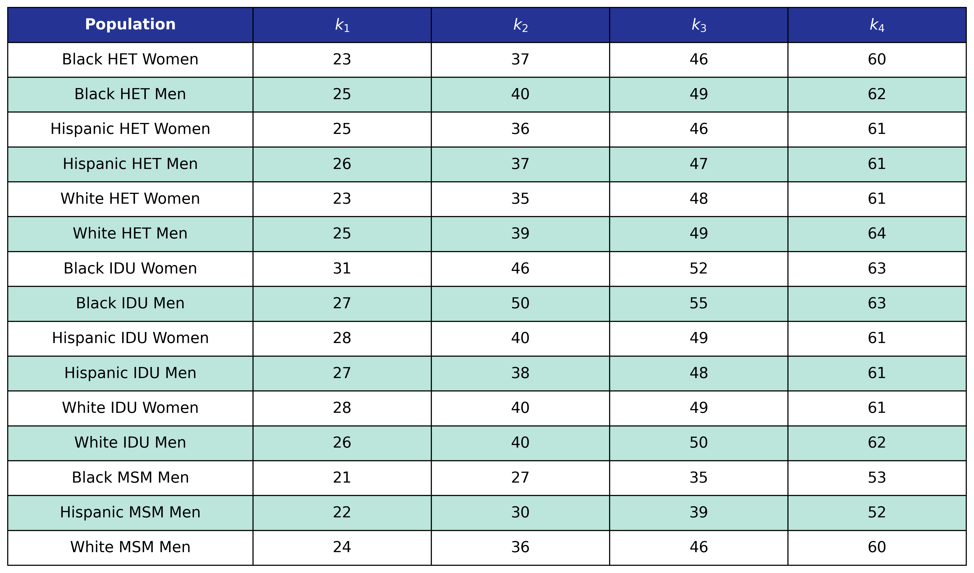
Table 28: Post-ART BMI Pre-ART CD4 Knots
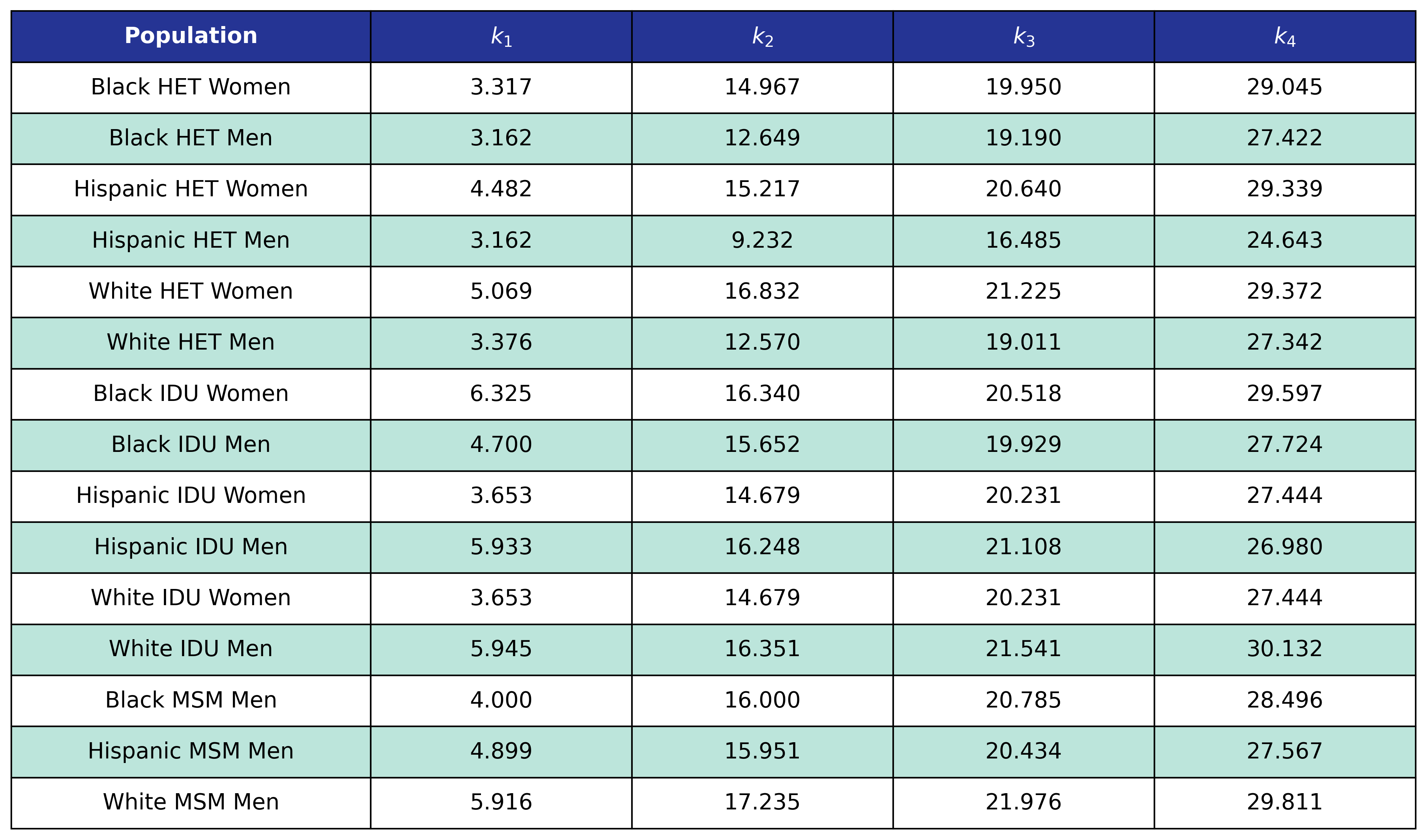
Table 28: Post-ART BMI Post-ART CD4 Knots
The estimates are as follows: