PEARL Model Overview </>
The PEARL (ProjEcting Age, multmoRbidity, and poLypharmacy) model is an agent-based simulation model of HIV care in the United States. The model leverages the power of the North American AIDS Cohort Collaboration on Research and Design (NA-ACCORD) data set. Data on ~200,000 HIV-infected individuals are provided by over 200 sites across North America. This size of this dataset allows us to treat 15 sub-populations independently. The PEARL model characterizes population by sex (male and female), race (white, black, and hispanic), and risk (men who have sex with men, intravenous drug users, and heterosexual HIV risk).
Table 1: Sub-Populations Used in the PEARL Model
| Population | Race | Risk | Sex | Code |
|---|---|---|---|---|
| Black Heterosexual Women | Black | HET | Female | het_black_female |
| Black Heterosexual Men | Black | HET | Male | het_black_male |
| Hispanic Heterosexual Women | Hispanic | HET | Female | het_hisp_female |
| Hispanic Heterosexual Men | Hispanic | HET | Male | het_hisp_male |
| White Heterosexual Women | White | HET | Female | het_white_female |
| White Heterosexual Men | White | HET | Male | het_white_male |
| Black Women Who Use Intravenous Drugs | Black | IDU | Female | idu_black_female |
| Black Men Who Use Intravenous Drugs | Black | IDU | Male | idu_black_male |
| Hispanic Women Who Use Intravenous Drugs | Hispanic | IDU | Female | idu_hisp_female |
| Hispanic Men Who Use Intravenous Drugs | Hispanic | IDU | Male | idu_hisp_male |
| White Women Who Use Intravenous Drugs | White | IDU | Female | idu_white_female |
| White Men Who Use Intravenous Drugs | White | IDU | Male | idu_white_male |
| Black Men Who Have Sex With Men | Black | MSM | Male | msm_black_male |
| Hispanic Men Who Have Sex With Men | Hispanic | MSM | Male | msm_hisp_male |
| White Men Who Have Sex With Men | White | MSM | Male | msm_white_male |
The PEARL model runs in discrete time steps representing one year. The simulations begin in year 2009 by creating an initial population of HIV-infected individuals receiving or disengaged from ART in the US. The size of this population and the distribution of their ages, ART initiation years, and CD4 count at ART initiation is estimated based on data available from NA-ACCORD and the Centers for Disease Control and Prevention (CDC). At the beginning of each simulated year (2010 – 2030), a population of those newly diagnosed with HIV enter the model, and a specific proportion (modeled as an increasing function of time) of these individuals link to HIV care and start ART. The population size, age, and CD4 count distributions at ART initiation are estimated from CDC’s and NA-ACCORD’s data. Individuals on ART experience a likelihood of mortality and disengagement from care over time. Upon disengagement, individuals experience an increase in probability of mortality and a gradual reduction in CD4 count. Time-varying CD4 count is updated for all individuals in the model depending on their HIV care status (i.e., increasing among those in care and decreasing among those out of care). All simulation parameters have been estimated from CDC’s and NA-ACCORD’s data for year 2010 to 2022. Simulated outcomes, in terms of age distribution of population in HIV care, are cross-validated against NA-ACCORD’s data during this period. Model projections are made from year 2023 to 2030.
Clarification on terminology: Given the complexities involved in defining, parametrizing and calibrating all steps of the HIV care continuum for the 15 sub-groups, we have limited the scope of the PEARL model to population of HIV infected individuals who have ever been and/or are currently on ART. Following this definition, the simulated population is divided into two groups including “ART users” (those currently on ART) and “ART non-users” (those previously on ART who disengaged from treatment and are currently off ART). Furthermore, the usage of term “HIV care” in this text is closely related to previous or current instances of “ART usage”, and does not include prior steps to ART initiation such as diagnosed, linked to care, retained, etc. We further underscore the difference in terminology used to refer to “population on ART” (those receiving ART in a given period of time, aka ART users), and “population initiating ART” (those starting ART for the first time, aka first time ART initiators) throughout the text.
Initial Population in Year 2009 </>
Population Size </>
The size of the initial sub-populations using ART in 2009 is estimated from CDC surveillance data through the Medical Monitoring Project (MMP).
First, the estimated number of persons living with HIV infection in 2009 for each sex and risk group combination is taken from table 14a in the 2013 HIV Surveillance Report. We then use table 17a in the 2010 HIV Surveillance Report to calculate the proportion of each risk/sex group by race. We multiply these two numbers to get an estimate of the total number of persons in each sub-population who are living with HIV.
Finally, we multiply the estimated number living with HIV by estimated proportion of that sub-population to be receiving ART treatment. These estimates come from different sources depending on the sub-population.
Table 2: Total ART Users in 2009
| Population | # With HIV Per Risk/Sex | Proportion By Race | # By Sub-Population | Proportion On ART | Total On ART In 2009 | ART Source |
|---|---|---|---|---|---|---|
| het_black_female | 148,349 | 0.613 | 90,981 | 0.514 | 46,764 | CDC MMWR, February 7, 2014, Table 3 |
| het_black_male | 65,857 | 0.632 | 41,608 | 0.421 | 17,516 | CDC MMWR, February 7, 2014, Table 3 |
| het_hisp_female | 148,349 | 0.191 | 28,342 | 0.498 | 14,114 | CDC MMWR, October 10, 2014, Table 3 |
| het_hisp_male | 65,857 | 0.212 | 13,940 | 0.459 | 6,398 | CDC MMWR, October 10, 2014, Table 3 |
| het_white_female | 148,349 | 0.167 | 24,742 | 0.551 | 13,632 | Correspondence with Luke Shouse, CDC |
| het_white_male | 65,857 | 0.131 | 8,635 | 0.37 | 3,194 | Correspondence with Luke Shouse, CDC |
| idu_black_female | 53,717 | 0.528 | 28,350 | 0.498 | 14,118 | CDC MMWR, February 7, 2014, Table 3 |
| idu_black_male | 134,962 | 0.429 | 57,881 | 0.34 | 19,679 | CDC MMWR, February 7, 2014, Table 3 |
| idu_hisp_female | 53,717 | 0.199 | 10,711 | 0.341 | 3,652 | CDC MMWR, October 10, 2014, Table 3 |
| idu_hisp_male | 134,962 | 0.270 | 36,391 | 0.31 | 11,281 | CDC MMWR, October 10, 2014, Table 3 |
| idu_white_female | 53,717 | 0.245 | 13,152 | 0.55 | 7,233 | Correspondence with Luke Shouse, CDC |
| idu_white_male | 134,962 | 0.275 | 37,145 | 0.455 | 16,900 | Correspondence with Luke Shouse, CDC |
| msm_black_male | 414,232 | 0.293 | 12,1240 | 0.471 | 57,104 | CDC MMWR, September 26, 2014, Table 3 |
| msm_hisp_male | 414,232 | 0.201 | 83,125 | 0.492 | 40,897 | CDC MMWR, September 26, 2014, Table 3 |
| msm_white_male | 414,232 | 0.474 | 196,500 | 0.496 | 97,464 | CDC MMWR, September 26, 2014, Table 3 |
Age Distribution </>
The age distribution of each sub-population was modeled using a two-component mixed normal distribution (resulting in the best fit among alternative models), as follows:
\[f(x|\lambda_1, \mu_1, \sigma_1, \mu_2, \sigma_2) = \lambda_1 g(x|\mu_1, \sigma_1) + (1 - \lambda_1)g(x|\mu_2, \sigma_2)\]where
\[g(x|\mu, \sigma) = \frac{1}{\sqrt{2\pi\sigma^2}}e^{-\frac{(x-\mu)^2}{2\sigma^2}}\]is just the normal distribution. Here $x$ is age of those on ART in year 2009, $\lambda_1$ is the mixing proportion, and the $\mu$’s and $\sigma$’s are the means and standard deviations of the bimodal distribution. These parameters (Table 3) were obtained by fitting to the NA-ACCORD population of ART users in 2009. The normalmixEM2comp function of the mixtools package for R was used to fit the distributions. When initializing a simulation run, the ages of the 2009 population were drawn from a distribution with the same parameters after being truncated at ages 18 and 85.
Table 3: Coefficients for Age of Initial Population
| group | lambda1 | mu1 | mu2 | sigma1 | sigma2 |
|---|---|---|---|---|---|
| het_black_female | 0.11 | 31.31 | 44.53 | 5.26 | 9.76 |
| het_black_male | 0.43 | 48.02 | 48.99 | 6.97 | 11.89 |
| het_hisp_female | 0.20 | 32.38 | 45.75 | 5.31 | 9.39 |
| het_hisp_male | 0.50 | 39.17 | 51.70 | 7.82 | 10.45 |
| het_white_female | 0.77 | 42.16 | 52.61 | 8.59 | 10.80 |
| het_white_male | 0.14 | 48.06 | 49.63 | 3.87 | 10.72 |
| idu_black_female | 0.17 | 42.62 | 50.18 | 8.31 | 6.49 |
| idu_black_male | 0.05 | 39.35 | 53.93 | 7.71 | 6.31 |
| idu_hisp_female | 0.08 | 29.98 | 48.81 | 2.85 | 7.09 |
| idu_hisp_male | 0.11 | 32.55 | 50.31 | 3.80 | 7.48 |
| idu_white_female | 0.07 | 33.64 | 45.92 | 4.28 | 8.24 |
| idu_white_male | 0.02 | 26.15 | 47.11 | 2.44 | 8.10 |
| msm_black_male | 0.12 | 25.68 | 45.00 | 3.34 | 9.41 |
| msm_hisp_male | 0.92 | 40.44 | 56.80 | 8.69 | 11.01 |
| msm_white_male | 0.15 | 46.26 | 46.92 | 3.40 | 10.54 |
Year of ART Initiation </>
To estimate the original year of ART initiation among the simulated population, we applied available data from the NA-ACCORD population on ART in year 2009. To this end, each sub-population was broken into the seven age categories, including <20, [20,30), [30,40), [40,50), [50,60), [60,70), $\geq$70. Within each category, we then estimated the proportion initiating ART in each year between 2000 and 2009 as shown in Table 4. Those initiating ART prior to 2000 were counted in the 2000 category. If there were no data from a given population in a certain age category, the proportions from the white MSM population were used as indicated by dashes in the following tables. We use the 2009 NA-ACCORD population to inform the ART initiation year of our starting population.
Table 4a: HET Female
| Race | Age Category | 2000 | 2001 | 2002 | 2003 | 2004 | 2005 | 2006 | 2007 | 2008 | 2009 |
|---|---|---|---|---|---|---|---|---|---|---|---|
| black | <20 | 0.17 | 0.00 | 0.00 | 0.00 | 0.00 | 0.00 | 0.00 | 0.00 | 0.50 | 0.33 |
| black | [20,30) | 0.03 | 0.02 | 0.02 | 0.03 | 0.03 | 0.10 | 0.14 | 0.15 | 0.22 | 0.26 |
| black | [30,40) | 0.17 | 0.05 | 0.05 | 0.08 | 0.09 | 0.09 | 0.12 | 0.10 | 0.13 | 0.12 |
| black | [40,50) | 0.27 | 0.07 | 0.05 | 0.07 | 0.07 | 0.08 | 0.08 | 0.10 | 0.10 | 0.10 |
| black | [50,60) | 0.28 | 0.07 | 0.05 | 0.08 | 0.08 | 0.08 | 0.08 | 0.09 | 0.11 | 0.09 |
| black | [60,70) | 0.30 | 0.07 | 0.04 | 0.07 | 0.09 | 0.07 | 0.05 | 0.06 | 0.15 | 0.11 |
| black | >=70 | 0.37 | 0.09 | 0.09 | 0.06 | 0.06 | 0.11 | 0.09 | 0.03 | 0.09 | 0.03 |
| hisp | <20 | 0.00 | 0.00 | 0.00 | 0.00 | 0.00 | 0.00 | 0.00 | 0.00 | 0.50 | 0.50 |
| hisp | [20,30) | 0.06 | 0.04 | 0.06 | 0.03 | 0.06 | 0.15 | 0.06 | 0.09 | 0.25 | 0.20 |
| hisp | [30,40) | 0.18 | 0.05 | 0.04 | 0.09 | 0.11 | 0.11 | 0.11 | 0.09 | 0.11 | 0.11 |
| hisp | [40,50) | 0.28 | 0.05 | 0.05 | 0.07 | 0.10 | 0.08 | 0.10 | 0.06 | 0.10 | 0.10 |
| hisp | [50,60) | 0.32 | 0.08 | 0.05 | 0.06 | 0.08 | 0.10 | 0.07 | 0.07 | 0.08 | 0.08 |
| hisp | [60,70) | 0.35 | 0.12 | 0.05 | 0.07 | 0.07 | 0.02 | 0.02 | 0.07 | 0.11 | 0.12 |
| hisp | >=70 | 1.00 | 0.00 | 0.00 | 0.00 | 0.00 | 0.00 | 0.00 | 0.00 | 0.00 | 0.00 |
| white | <20 | 0.00 | 0.00 | 0.00 | 0.00 | 0.00 | 0.00 | 0.00 | 0.00 | 0.50 | 0.50 |
| white | [20,30) | 0.04 | 0.04 | 0.02 | 0.00 | 0.10 | 0.17 | 0.10 | 0.10 | 0.17 | 0.25 |
| white | [30,40) | 0.26 | 0.04 | 0.07 | 0.07 | 0.10 | 0.07 | 0.07 | 0.09 | 0.08 | 0.14 |
| white | [40,50) | 0.42 | 0.05 | 0.06 | 0.04 | 0.09 | 0.05 | 0.07 | 0.07 | 0.08 | 0.08 |
| white | [50,60) | 0.47 | 0.03 | 0.05 | 0.03 | 0.06 | 0.07 | 0.03 | 0.07 | 0.09 | 0.11 |
| white | [60,70) | 0.47 | 0.05 | 0.07 | 0.08 | 0.08 | 0.02 | 0.03 | 0.07 | 0.08 | 0.05 |
| white | >=70 | 0.25 | 0.17 | 0.17 | 0.08 | 0.08 | 0.00 | 0.08 | 0.00 | 0.08 | 0.08 |
Table 4b: HET Male
| Race | Age Category | 2000 | 2001 | 2002 | 2003 | 2004 | 2005 | 2006 | 2007 | 2008 | 2009 |
|---|---|---|---|---|---|---|---|---|---|---|---|
| black | <20 | 0.50 | 0.00 | 0.00 | 0.00 | 0.00 | 0.00 | 0.00 | 0.00 | 0.50 | 0.00 |
| black | [20,30) | 0.02 | 0.03 | 0.02 | 0.02 | 0.03 | 0.13 | 0.11 | 0.17 | 0.18 | 0.26 |
| black | [30,40) | 0.12 | 0.05 | 0.03 | 0.05 | 0.10 | 0.09 | 0.12 | 0.11 | 0.17 | 0.17 |
| black | [40,50) | 0.26 | 0.07 | 0.05 | 0.07 | 0.07 | 0.09 | 0.08 | 0.08 | 0.10 | 0.13 |
| black | [50,60) | 0.36 | 0.06 | 0.05 | 0.07 | 0.07 | 0.07 | 0.08 | 0.08 | 0.08 | 0.08 |
| black | [60,70) | 0.40 | 0.09 | 0.07 | 0.05 | 0.09 | 0.07 | 0.06 | 0.07 | 0.05 | 0.06 |
| black | >=70 | 0.55 | 0.08 | 0.06 | 0.07 | 0.02 | 0.01 | 0.08 | 0.05 | 0.06 | 0.03 |
| hisp | <20 | – | – | – | – | – | – | – | – | – | – |
| hisp | [20,30) | 0.01 | 0.01 | 0.03 | 0.01 | 0.04 | 0.06 | 0.11 | 0.14 | 0.26 | 0.32 |
| hisp | [30,40) | 0.11 | 0.05 | 0.06 | 0.06 | 0.10 | 0.10 | 0.10 | 0.10 | 0.19 | 0.13 |
| hisp | [40,50) | 0.26 | 0.05 | 0.04 | 0.09 | 0.08 | 0.11 | 0.08 | 0.08 | 0.10 | 0.09 |
| hisp | [50,60) | 0.38 | 0.05 | 0.04 | 0.06 | 0.06 | 0.07 | 0.05 | 0.09 | 0.12 | 0.07 |
| hisp | [60,70) | 0.46 | 0.08 | 0.05 | 0.09 | 0.04 | 0.08 | 0.10 | 0.04 | 0.04 | 0.02 |
| hisp | >=70 | 0.52 | 0.12 | 0.04 | 0.04 | 0.08 | 0.00 | 0.04 | 0.00 | 0.12 | 0.04 |
| white | <20 | – | – | – | – | – | – | – | – | – | – |
| white | [20,30) | 0.00 | 0.00 | 0.00 | 0.00 | 0.15 | 0.23 | 0.00 | 0.00 | 0.31 | 0.31 |
| white | [30,40) | 0.18 | 0.01 | 0.04 | 0.03 | 0.08 | 0.06 | 0.09 | 0.16 | 0.22 | 0.13 |
| white | [40,50) | 0.37 | 0.04 | 0.06 | 0.06 | 0.10 | 0.05 | 0.08 | 0.07 | 0.09 | 0.09 |
| white | [50,60) | 0.40 | 0.06 | 0.08 | 0.06 | 0.09 | 0.06 | 0.05 | 0.06 | 0.08 | 0.06 |
| white | [60,70) | 0.49 | 0.04 | 0.04 | 0.11 | 0.05 | 0.07 | 0.05 | 0.04 | 0.08 | 0.02 |
| white | >=70 | 0.50 | 0.12 | 0.08 | 0.00 | 0.08 | 0.00 | 0.04 | 0.08 | 0.04 | 0.04 |
Table 4c: IDU Female
| Race | Age Category | 2000 | 2001 | 2002 | 2003 | 2004 | 2005 | 2006 | 2007 | 2008 | 2009 |
|---|---|---|---|---|---|---|---|---|---|---|---|
| black | <20 | – | – | – | – | – | – | – | – | – | – |
| black | [20,30) | 0.00 | 0.00 | 0.00 | 0.00 | 0.00 | 0.17 | 0.17 | 0.50 | 0.00 | 0.17 |
| black | [30,40) | 0.14 | 0.07 | 0.10 | 0.12 | 0.00 | 0.10 | 0.10 | 0.12 | 0.14 | 0.12 |
| black | [40,50) | 0.33 | 0.07 | 0.05 | 0.07 | 0.06 | 0.09 | 0.05 | 0.09 | 0.12 | 0.08 |
| black | [50,60) | 0.42 | 0.09 | 0.03 | 0.05 | 0.05 | 0.06 | 0.09 | 0.07 | 0.06 | 0.08 |
| black | [60,70) | 0.31 | 0.00 | 0.06 | 0.12 | 0.06 | 0.12 | 0.03 | 0.06 | 0.09 | 0.12 |
| black | >=70 | – | – | – | – | – | – | – | – | – | – |
| hisp | <20 | – | – | – | – | – | – | – | – | – | – |
| hisp | [20,30) | 0.00 | 0.00 | 0.00 | 0.00 | 0.20 | 0.00 | 0.00 | 0.60 | 0.00 | 0.20 |
| hisp | [30,40) | 0.20 | 0.00 | 0.20 | 0.00 | 0.07 | 0.00 | 0.13 | 0.00 | 0.20 | 0.20 |
| hisp | [40,50) | 0.24 | 0.06 | 0.02 | 0.10 | 0.06 | 0.12 | 0.08 | 0.18 | 0.10 | 0.06 |
| hisp | [50,60) | 0.39 | 0.04 | 0.04 | 0.13 | 0.04 | 0.07 | 0.04 | 0.07 | 0.09 | 0.09 |
| hisp | [60,70) | 0.33 | 0.00 | 0.17 | 0.00 | 0.00 | 0.00 | 0.00 | 0.00 | 0.17 | 0.33 |
| hisp | >=70 | 0.00 | 0.00 | 0.00 | 0.00 | 1.00 | 0.00 | 0.00 | 0.00 | 0.00 | 0.00 |
| white | <20 | – | – | – | – | – | – | – | – | – | – |
| white | [20,30) | 0.20 | 0.00 | 0.00 | 0.00 | 0.00 | 0.10 | 0.00 | 0.20 | 0.00 | 0.50 |
| white | [30,40) | 0.23 | 0.03 | 0.10 | 0.06 | 0.11 | 0.10 | 0.01 | 0.08 | 0.21 | 0.07 |
| white | [40,50) | 0.34 | 0.05 | 0.06 | 0.09 | 0.12 | 0.06 | 0.09 | 0.04 | 0.07 | 0.08 |
| white | [50,60) | 0.40 | 0.07 | 0.07 | 0.08 | 0.07 | 0.05 | 0.04 | 0.04 | 0.11 | 0.08 |
| white | [60,70) | 0.36 | 0.00 | 0.00 | 0.18 | 0.00 | 0.00 | 0.18 | 0.00 | 0.18 | 0.09 |
| white | >=70 | 0.50 | 0.00 | 0.00 | 0.00 | 0.00 | 0.00 | 0.00 | 0.50 | 0.00 | 0.00 |
Table 4d: IDU Male
| Race | Age Category | 2000 | 2001 | 2002 | 2003 | 2004 | 2005 | 2006 | 2007 | 2008 | 2009 |
|---|---|---|---|---|---|---|---|---|---|---|---|
| black | <20 | – | – | – | – | – | – | – | – | – | – |
| black | [20,30) | 0.11 | 0.00 | 0.11 | 0.00 | 0.00 | 0.00 | 0.11 | 0.22 | 0.22 | 0.22 |
| black | [30,40) | 0.19 | 0.00 | 0.06 | 0.04 | 0.15 | 0.06 | 0.09 | 0.13 | 0.13 | 0.15 |
| black | [40,50) | 0.36 | 0.06 | 0.05 | 0.09 | 0.05 | 0.08 | 0.08 | 0.08 | 0.07 | 0.07 |
| black | [50,60) | 0.51 | 0.05 | 0.06 | 0.06 | 0.06 | 0.04 | 0.06 | 0.06 | 0.05 | 0.05 |
| black | [60,70) | 0.61 | 0.06 | 0.02 | 0.04 | 0.05 | 0.03 | 0.05 | 0.04 | 0.03 | 0.07 |
| black | >=70 | 0.62 | 0.00 | 0.00 | 0.06 | 0.06 | 0.06 | 0.12 | 0.06 | 0.00 | 0.00 |
| hisp | <20 | – | – | – | – | – | – | – | – | – | – |
| hisp | [20,30) | 0.00 | 0.00 | 0.00 | 0.00 | 0.07 | 0.00 | 0.14 | 0.29 | 0.29 | 0.21 |
| hisp | [30,40) | 0.14 | 0.03 | 0.06 | 0.03 | 0.07 | 0.19 | 0.08 | 0.10 | 0.15 | 0.14 |
| hisp | [40,50) | 0.34 | 0.05 | 0.03 | 0.06 | 0.06 | 0.08 | 0.09 | 0.13 | 0.10 | 0.07 |
| hisp | [50,60) | 0.48 | 0.06 | 0.05 | 0.04 | 0.06 | 0.04 | 0.05 | 0.10 | 0.06 | 0.06 |
| hisp | [60,70) | 0.52 | 0.04 | 0.06 | 0.06 | 0.08 | 0.08 | 0.00 | 0.06 | 0.06 | 0.02 |
| hisp | >=70 | 0.67 | 0.00 | 0.00 | 0.00 | 0.00 | 0.00 | 0.00 | 0.33 | 0.00 | 0.00 |
| white | <20 | – | – | – | – | – | – | – | – | – | – |
| white | [20,30) | 0.00 | 0.02 | 0.02 | 0.00 | 0.00 | 0.13 | 0.13 | 0.15 | 0.26 | 0.30 |
| white | [30,40) | 0.15 | 0.06 | 0.04 | 0.04 | 0.07 | 0.08 | 0.10 | 0.19 | 0.13 | 0.14 |
| white | [40,50) | 0.42 | 0.06 | 0.04 | 0.06 | 0.07 | 0.08 | 0.07 | 0.07 | 0.07 | 0.08 |
| white | [50,60) | 0.51 | 0.07 | 0.05 | 0.06 | 0.05 | 0.04 | 0.05 | 0.05 | 0.07 | 0.05 |
| white | [60,70) | 0.68 | 0.00 | 0.05 | 0.07 | 0.06 | 0.06 | 0.01 | 0.02 | 0.01 | 0.05 |
| white | >=70 | 0.50 | 0.25 | 0.25 | 0.00 | 0.00 | 0.00 | 0.00 | 0.00 | 0.00 | 0.00 |
Table 4e: MSM
| Race | Age Category | 2000 | 2001 | 2002 | 2003 | 2004 | 2005 | 2006 | 2007 | 2008 | 2009 |
|---|---|---|---|---|---|---|---|---|---|---|---|
| black | <20 | 0.00 | 0.00 | 0.00 | 0.00 | 0.00 | 0.00 | 0.00 | 0.00 | 0.00 | 1.00 |
| black | [20,30) | 0.01 | 0.01 | 0.02 | 0.02 | 0.05 | 0.07 | 0.08 | 0.14 | 0.26 | 0.34 |
| black | [30,40) | 0.17 | 0.05 | 0.06 | 0.06 | 0.08 | 0.07 | 0.10 | 0.12 | 0.14 | 0.16 |
| black | [40,50) | 0.38 | 0.06 | 0.05 | 0.07 | 0.06 | 0.06 | 0.07 | 0.07 | 0.09 | 0.08 |
| black | [50,60) | 0.47 | 0.07 | 0.05 | 0.07 | 0.06 | 0.05 | 0.06 | 0.06 | 0.04 | 0.07 |
| black | [60,70) | 0.59 | 0.06 | 0.07 | 0.05 | 0.05 | 0.04 | 0.03 | 0.03 | 0.05 | 0.04 |
| black | >=70 | 0.56 | 0.03 | 0.12 | 0.00 | 0.03 | 0.12 | 0.00 | 0.03 | 0.06 | 0.03 |
| hisp | <20 | 0.00 | 0.00 | 0.00 | 0.00 | 0.00 | 0.00 | 0.00 | 0.00 | 0.25 | 0.75 |
| hisp | [20,30) | 0.00 | 0.00 | 0.01 | 0.02 | 0.04 | 0.07 | 0.10 | 0.16 | 0.21 | 0.39 |
| hisp | [30,40) | 0.13 | 0.03 | 0.04 | 0.06 | 0.09 | 0.09 | 0.11 | 0.12 | 0.14 | 0.19 |
| hisp | [40,50) | 0.28 | 0.07 | 0.06 | 0.07 | 0.06 | 0.09 | 0.08 | 0.09 | 0.10 | 0.11 |
| hisp | [50,60) | 0.41 | 0.08 | 0.05 | 0.04 | 0.07 | 0.05 | 0.07 | 0.09 | 0.09 | 0.05 |
| hisp | [60,70) | 0.56 | 0.06 | 0.05 | 0.07 | 0.04 | 0.02 | 0.04 | 0.02 | 0.07 | 0.06 |
| hisp | >=70 | 0.61 | 0.00 | 0.04 | 0.09 | 0.00 | 0.09 | 0.09 | 0.00 | 0.04 | 0.04 |
| white | <20 | 0.00 | 0.00 | 0.00 | 0.00 | 0.00 | 0.00 | 0.00 | 0.00 | 0.00 | 1.00 |
| white | [20,30) | 0.01 | 0.02 | 0.01 | 0.02 | 0.04 | 0.06 | 0.09 | 0.16 | 0.24 | 0.35 |
| white | [30,40) | 0.14 | 0.04 | 0.04 | 0.05 | 0.08 | 0.08 | 0.10 | 0.13 | 0.15 | 0.18 |
| white | [40,50) | 0.39 | 0.05 | 0.04 | 0.06 | 0.06 | 0.06 | 0.08 | 0.07 | 0.08 | 0.09 |
| white | [50,60) | 0.51 | 0.05 | 0.04 | 0.05 | 0.06 | 0.05 | 0.06 | 0.06 | 0.07 | 0.05 |
| white | [60,70) | 0.60 | 0.06 | 0.05 | 0.05 | 0.04 | 0.03 | 0.05 | 0.05 | 0.03 | 0.04 |
| white | >=70 | 0.64 | 0.05 | 0.03 | 0.05 | 0.09 | 0.05 | 0.03 | 0.03 | 0.02 | 0.01 |
CD4 Count at ART Initiation </>
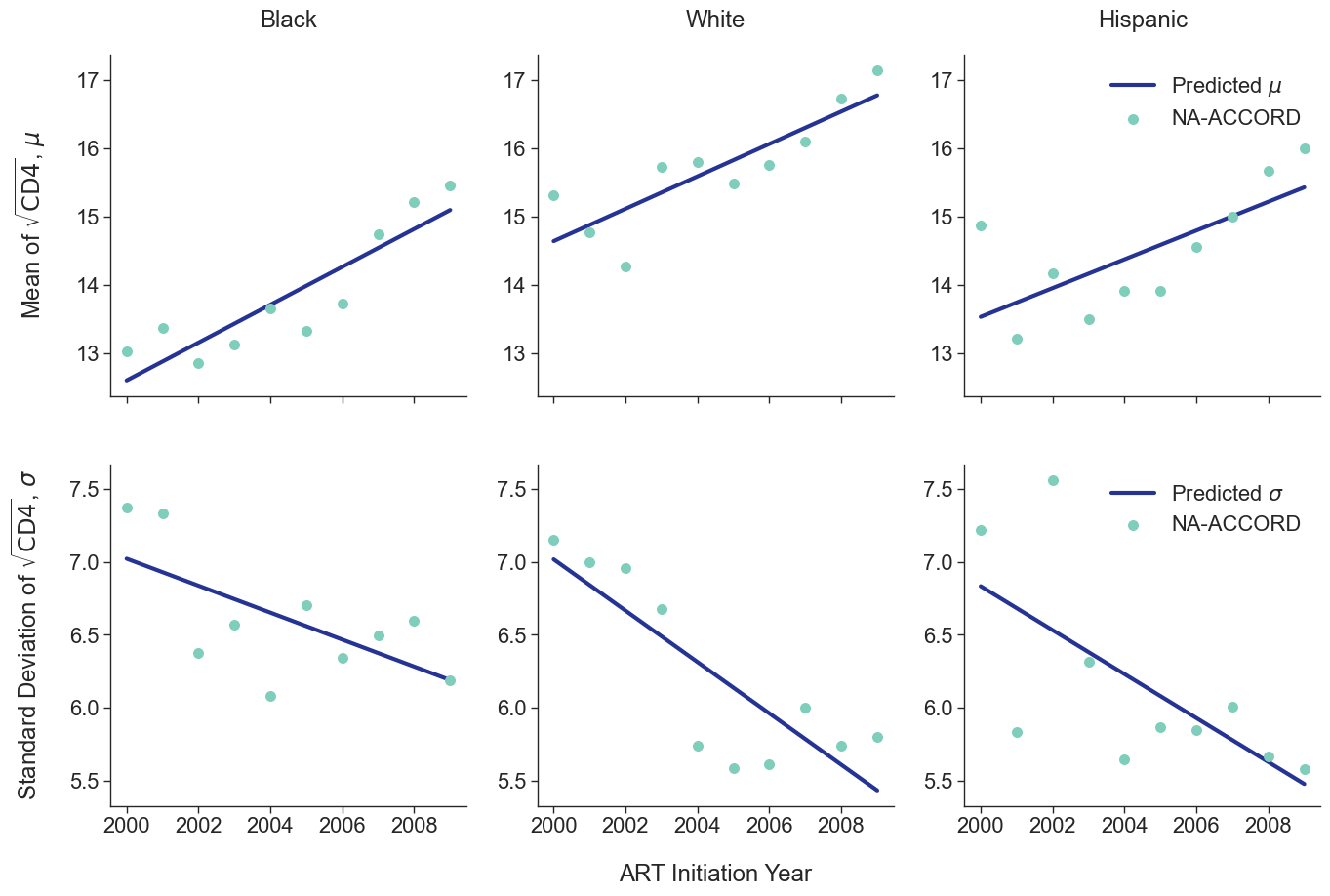
To estimate the CD4 count at first ART initiation among simulated population in year 2009, we applied available data from the NA-ACCORD population on ART in year 2009. To this end, each sub-population was split into original ART initiation years between [2000, 2009] as estimated in the previous step. A normal distribution was fit to describe the \(\sqrt{\mathrm{CD4}}\) count at ART initiation in each year. Within each sub-population, a linear regression model was applied to describe changes in the normal distribution parameters (\(\mu\) mean and \(\sigma\) standard deviation) over time, such that
\[\mu(\mathrm{year}) = \mu_0 + \beta_\mu \cdot \mathrm{year}\]and
\[\sigma(\mathrm{year}) = \sigma_0 + \beta_\sigma \cdot \mathrm{year}\]The linear regression was fit using the glm function of the stats package in base R. Table 5 presents the value of the fitted coefficients.
Table 5: Initial Population CD4 Count at ART Initiation Coefficients
| group | meanint | meanslp | stdint | stdslp |
|---|---|---|---|---|
| het_black_female | -388.48 | 0.20 | 108.83 | -0.05 |
| idu_black_male | -20.03 | 0.02 | 117.09 | -0.06 |
| idu_hisp_male | 110.09 | -0.05 | -54.13 | 0.03 |
| msm_black_male | -450.86 | 0.23 | 183.12 | -0.09 |
| idu_white_male | -239.51 | 0.13 | 152.97 | -0.07 |
| het_hisp_female | -127.64 | 0.07 | -37.09 | 0.02 |
| het_black_male | 14.98 | 0.00 | 151.32 | -0.07 |
| het_hisp_male | 50.88 | -0.02 | 132.09 | -0.06 |
| msm_hisp_male | -506.13 | 0.26 | 243.24 | -0.12 |
| idu_black_female | -261.53 | 0.14 | 194.90 | -0.09 |
| msm_white_male | -339.98 | 0.18 | 375.69 | -0.18 |
| het_white_male | -584.30 | 0.30 | 155.80 | -0.07 |
| idu_hisp_female | -222.97 | 0.12 | 602.42 | -0.30 |
| het_white_female | -320.81 | 0.17 | 302.93 | -0.15 |
| idu_white_female | -294.14 | 0.15 | -583.75 | 0.29 |
When drawing CD4 values, we truncate the normal distribution at $0$ and $\sqrt{2000}$. The trajectory of the means and standard deviations is shown in the following plots:
Figure 1a: HET Female
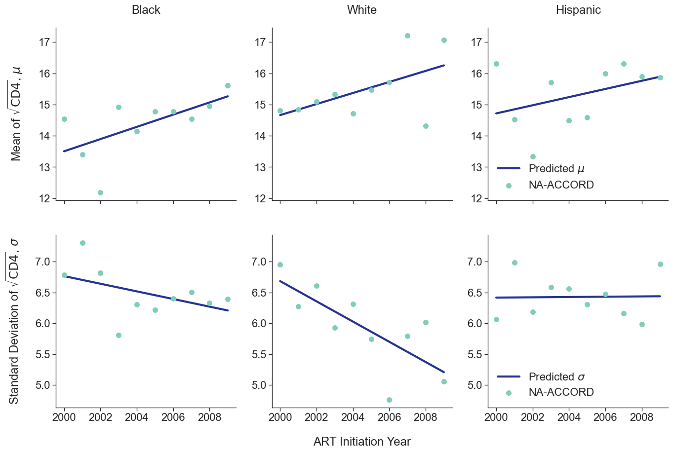
Figure 1b: HET Male
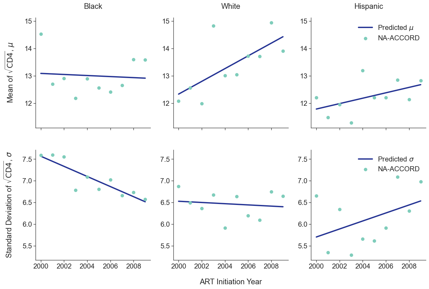
Figure 1c: IDU Female
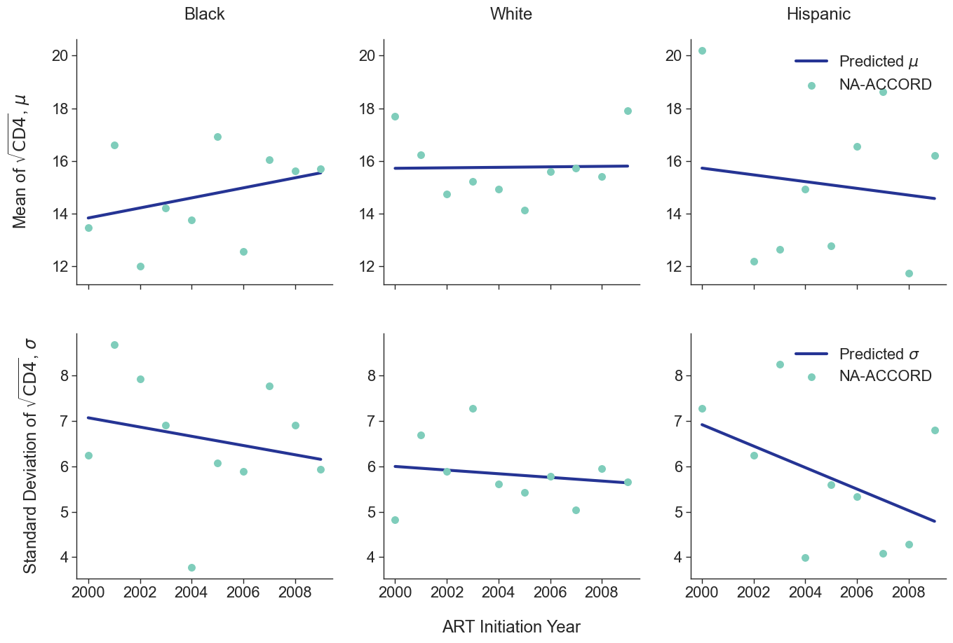
Figure 1d: IDU Male
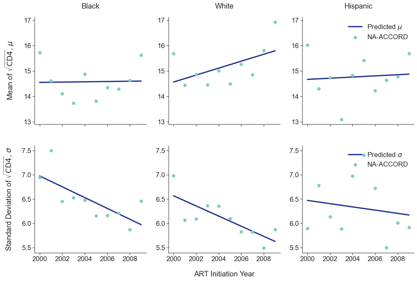
Figure 1e: MSM
Initial Population not Using ART in Year 2009 </>
In addition to an initial population of people on ART in 2009 the simulation is seeded with an initial population of those who had previously been on ART but are currently disengaged from care (and experience a likelihood of ART re-engagement in year 2010 and afterward). The size of this population is generated by estimating the number of those linking to care but not initiating ART from 2006 to 2009 as outlined in the following section. The age and CD4 count distributions for this population is assumed to be identical to the initial ART using population.
Population Initiating ART From 2010 - 2030 </>
Population Size of ART Initiators </>
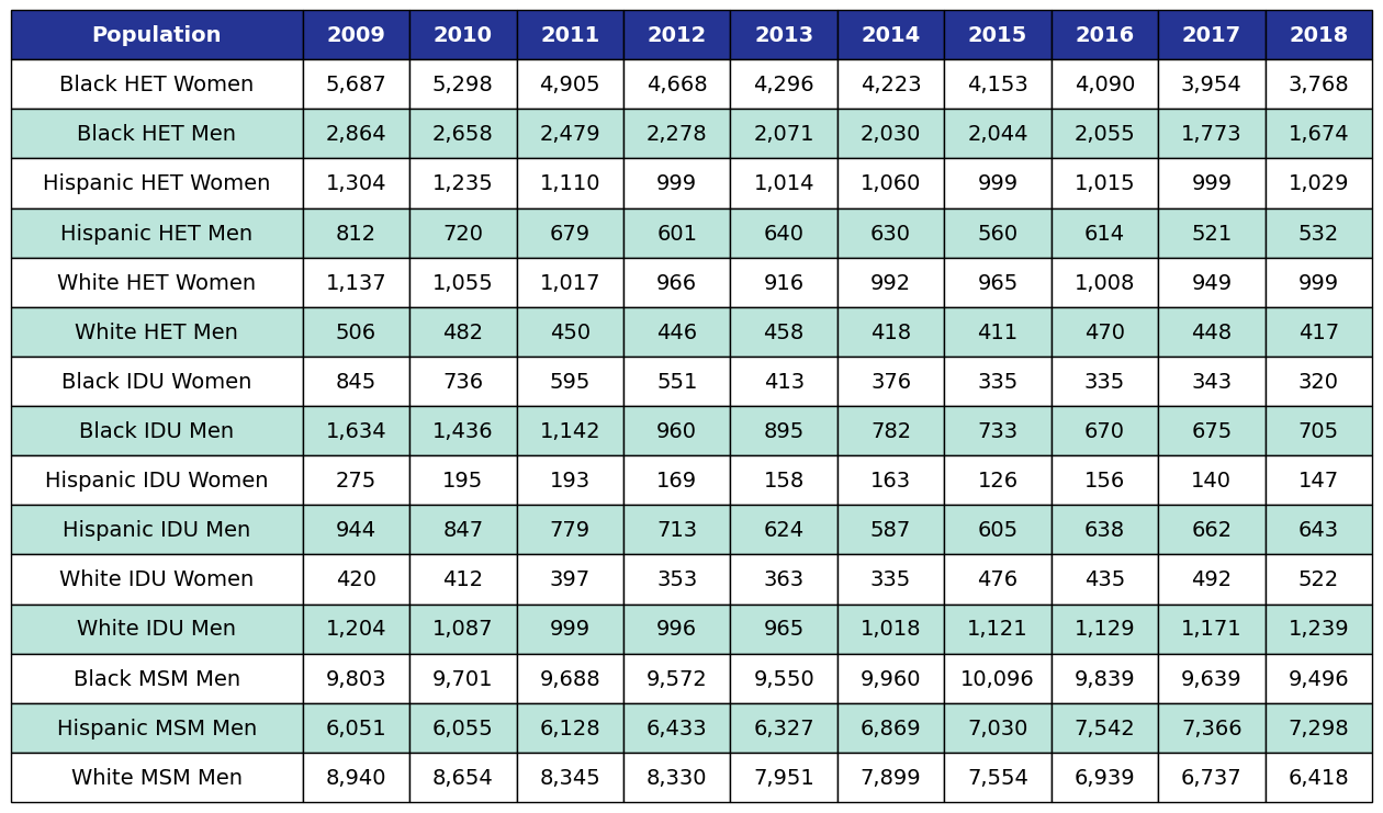
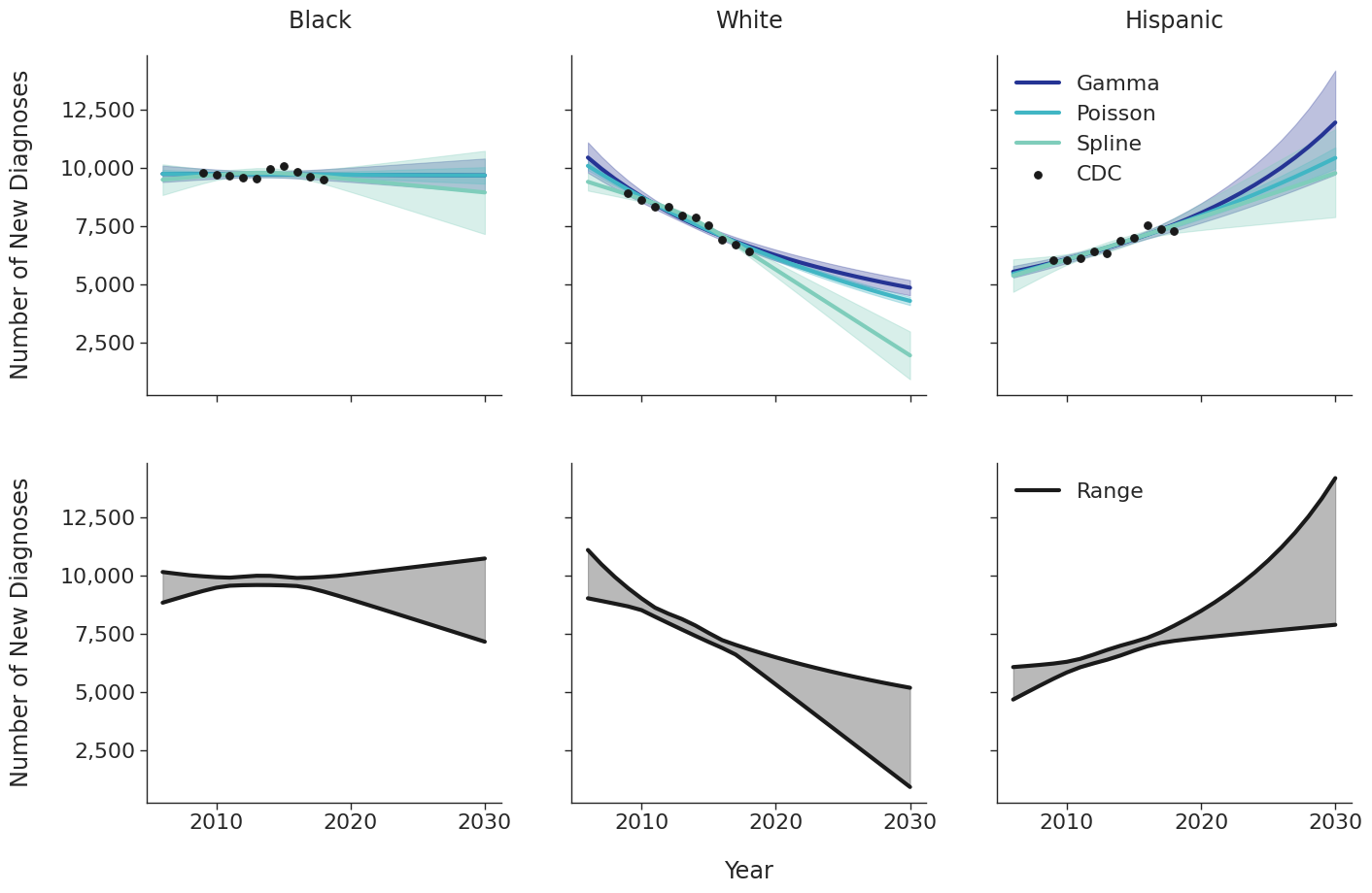
New HIV diagnosis: In order to predict the number of new people linking to HIV care and starting ART in a given year, we begin with data on the number of new HIV diagnoses per year as estimated by the CDC’s Medical Monitoring Project (MMP) as shown in Table 6. Dates before 2016 came from Table 1 of the 2015 HIV Surveillance Report, while data 2016 and after came from Table 1 of the 2018 HIV Surveillance Report.
Table 6: Number of New HIV Diagnoses by Year
Various candidate models were proposed in order to predict the number of new HIV diagnoses from 2006 to 2030. Predicted HIV diagnoses prior to 2010 are used later in the initial 2009 population creation. After removing models with inadequate fit (based on AIC values), the data were fit using a Poisson model, a gamma model and a natural cubic spline model with a single knot. Of these models, those resulting in unrealistic projections (>50% increase in new diagnosis from 2020 – 2030) were also removed. The Poisson and gamma fits were accomplished using the glm function of the stats package in base R, while the spline fit was generated using the lm and ns functions of the base R packages stats and splines, respectively. To incorporate additional uncertainties in annual estimates, the 95% prediction intervals around each fit were calculated. These prediction intervals were combined to generate an annual range for the number of new diagnosis in each year for a given subgroup (black, white and Hispanic). The annual ranges are estimated from the largest upper prediction interval and the lowest lower prediction interval of existing models as shown in panel 2 of Figure 2. For each simulation run, a random number between 0 and 1 is drawn that defines the number of new diagnoses in that simulation. Figure 2 shows the full ranges used to generate the number of new diagnoses.
Figure 2a: HET Female
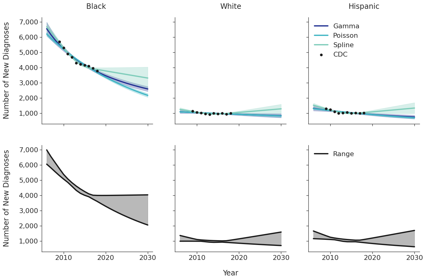
Figure 2b: HET Male
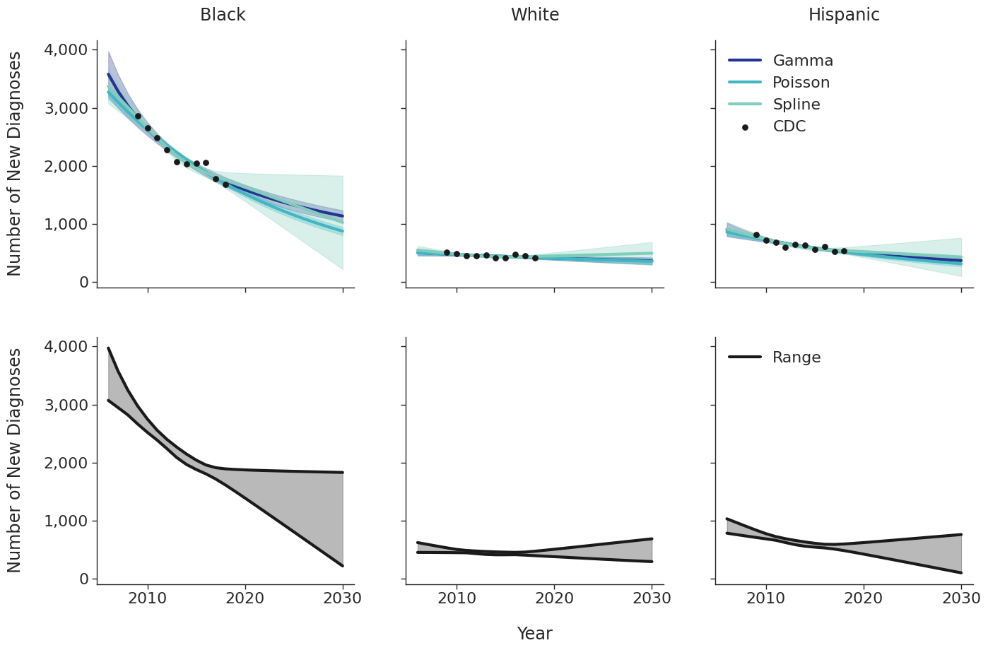
Figure 2c: IDU Female
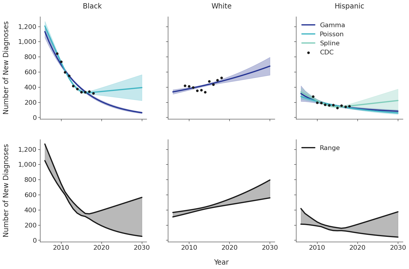
Figure 2d: IDU Male
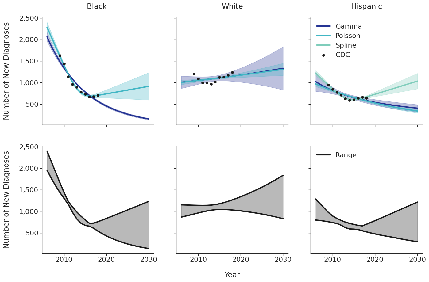
Figure 2e: MSM
Linkage to HIV care and ART initiation: We estimated percentage of people in each sub-population linking to HIV care in the first 4 months after HIV diagnosis for each year between 2010 – 2015 from the CDC. To project future trends from 2016 to 2030, we applied a linear regression and capped at 95% linkage as shown in Figure 3. The linear regression was accomplished using the ols function of the statsmodels package for Python. Among remaining cases, we further assumed that 40% link to care over the next three years after initial diagnosis. To estimate the population starting ART, we assumed that 70% of those linking to care begin ART immediately in years prior to 2011. This percentage rises to 85% in 2011 and up to 97% thereafter.
Figure 3a: HET Female
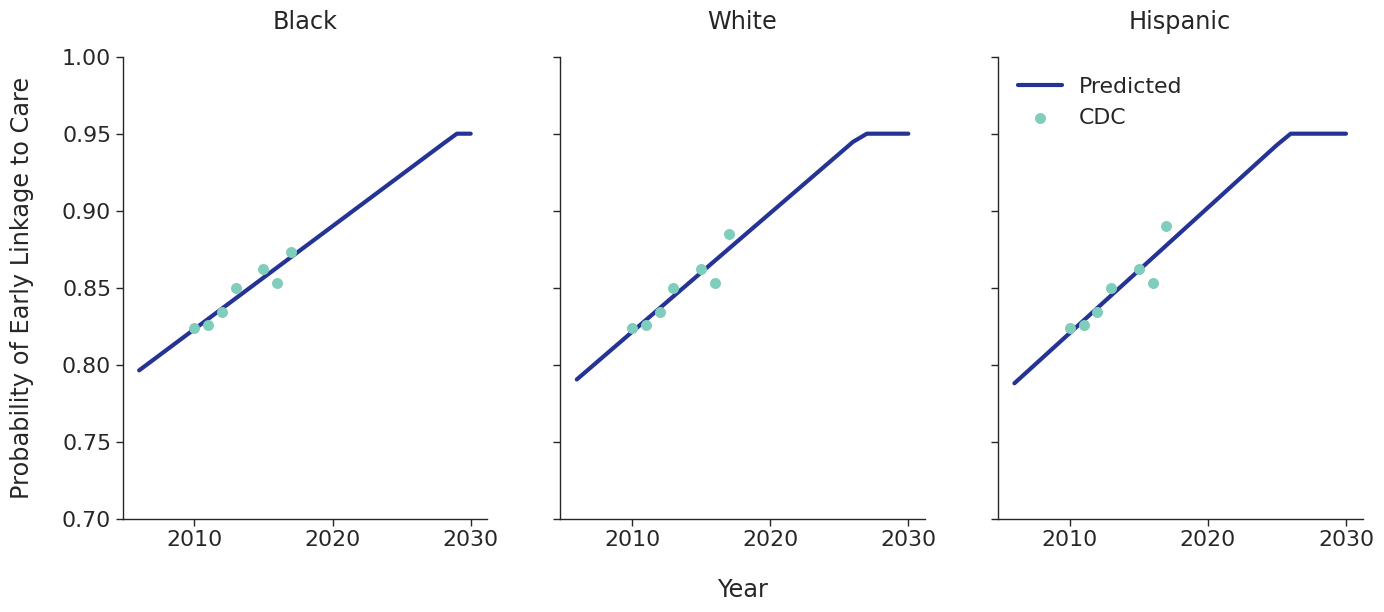
Figure 3b: HET Male
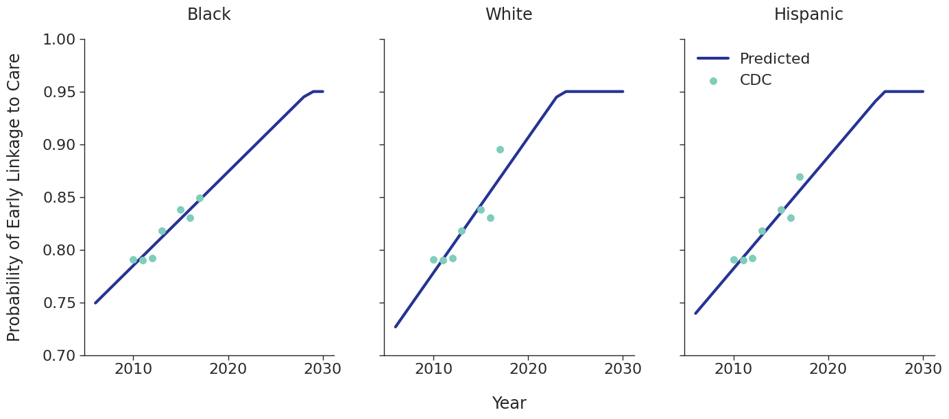
Figure 3c: IDU Female
Figure 3d: IDU Male
Figure 3e: MSM
Age Distribution of ART Initiators </>
The age distributions of the populations initiating ART in each year are modeled as a two component mixed normal distribution:
\[f(x|\lambda_1, \mu_1, \sigma_1, \mu_2, \sigma_2) = \lambda_1 g(x|\mu_1, \sigma_1) + (1 - \lambda_1)g(x|\mu_2, \sigma_2)\]where
\[g(x|\mu, \sigma) = \frac{1}{\sqrt{2\pi\sigma^2}}e^{-\frac{(x-\mu)^2}{2\sigma^2}}\]is the usual normal distribution. Here $x$ represents age at ART initiation, $\lambda_1$ is the mixing proportion, and the $\mu$’s and $\sigma$’s are the means and standard deviations of the bimodal distribution. A fit was found for each ART initiation year, from 2010 to 2022, and each sub-population using data from NA-ACCORD using the normalmixEM function of the mixtools package for R. Due to lack of available data, some years had to be collapsed together according to the following rules:
Age Distribution Data Collapse Rules
Heterosexual Hispanic Female:
-
2015-2017
-
2018-2022
Heterosexual Hispanic Male :
-
2016-2017
-
2018-2022
Heterosexual White Female:
-
2015-2016
-
2017-2018
-
2019-2022
Heterosexual White Male:
-
2016-2017
-
2018-2019
-
2020-2022
IDU Black Female:
-
2010-2013
-
2014-2022
IDU Black Male:
-
2015-2016
-
2017-2018
-
2019-2022
IDU Hisp Female:
- 2010-2022
IDU Hisp Male:
-
2010-2011
-
2012-2013
-
2014-2015
-
2016-2022
IDU White Female:
-
2010-2011
-
2012-2014
-
2015-2022
IDU White Male:
-
2018-2019
-
2020-2022
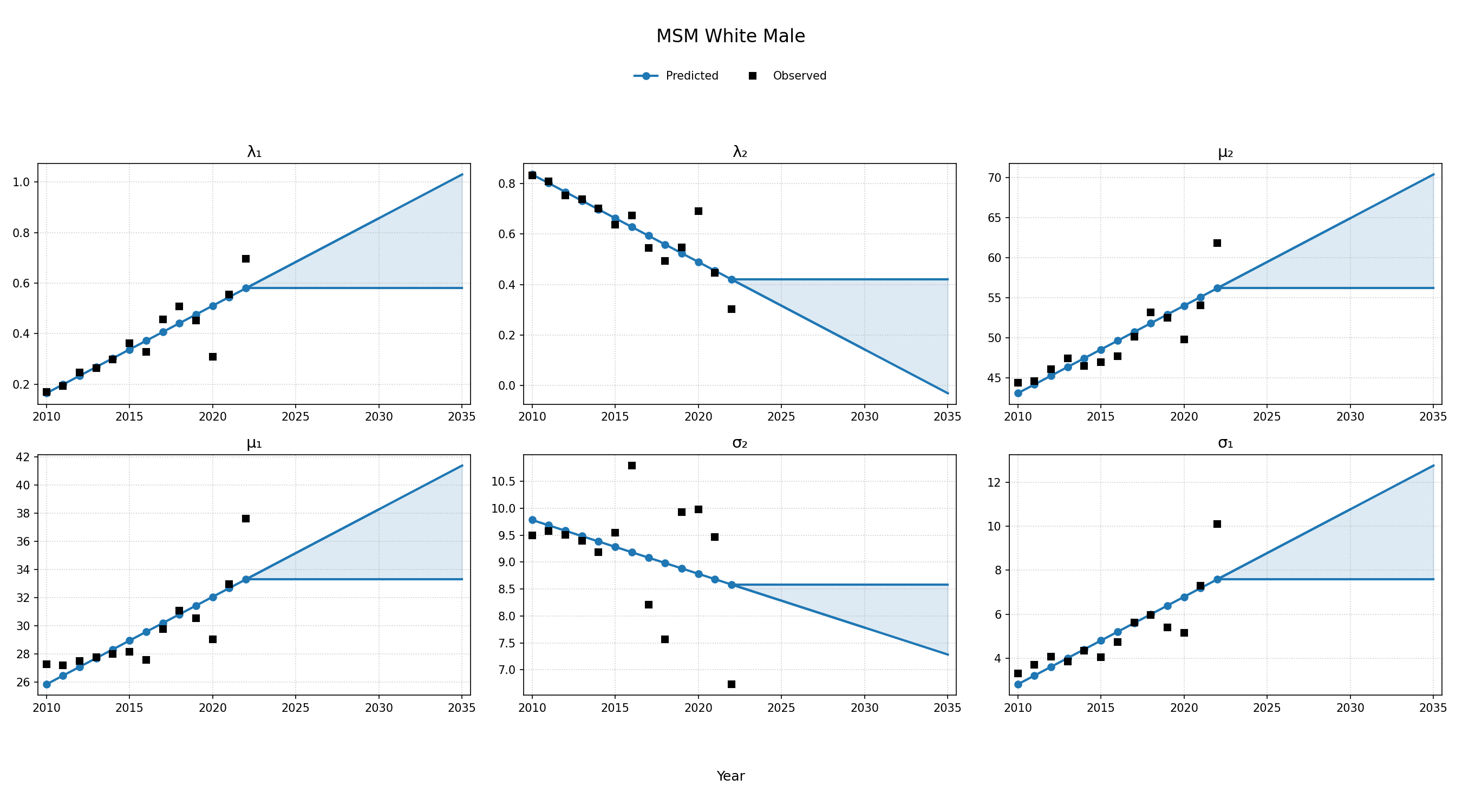
To estimate changes in age distribution of ART initiators over time, we modeled changes in the five parameters of the distribution as a linear function of calendar year (Figure 4). For this purpose, each parameter was fit to a linear regression using the glm function of the stats package in base R (blue dots in Figure 4). Given the sharp rate of change through the linear fit and lack of available data to support predictions from 2018 onward, the predicted values in year 2018 were used as an upper/lower bound to develop a prediction range for future years (shaded areas in Figure 4). Values for \(\lambda_1\) were truncated between 0 and 1 and all variables are truncated at 0. These models were applied to generate the value of 5 parameters describing the bimodal normal distribution of age at ART initiation in each year. The distribution was further truncated at ages 18 and 85.
Figure 4a: HET Black Female
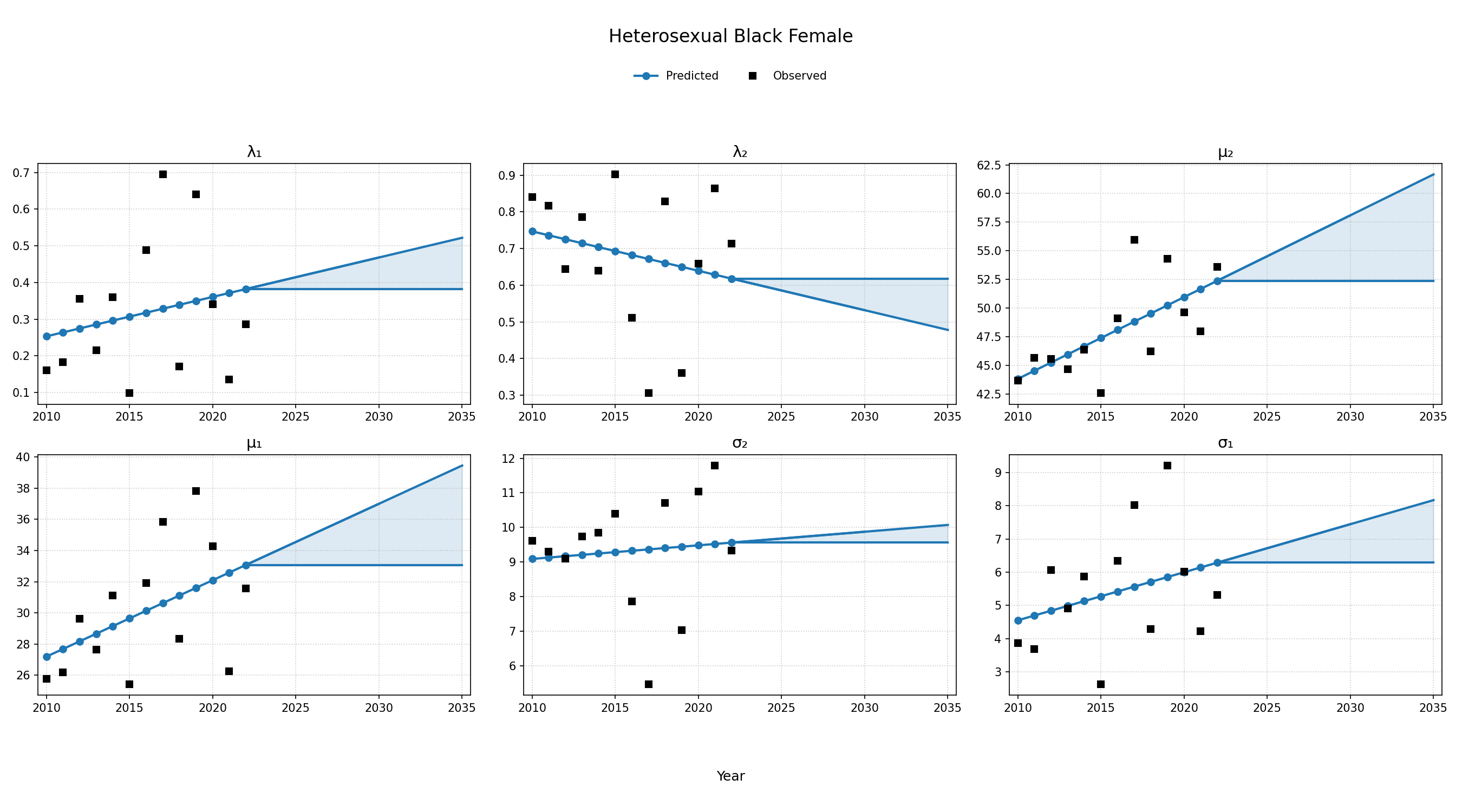
Figure 4b: HET Black Male
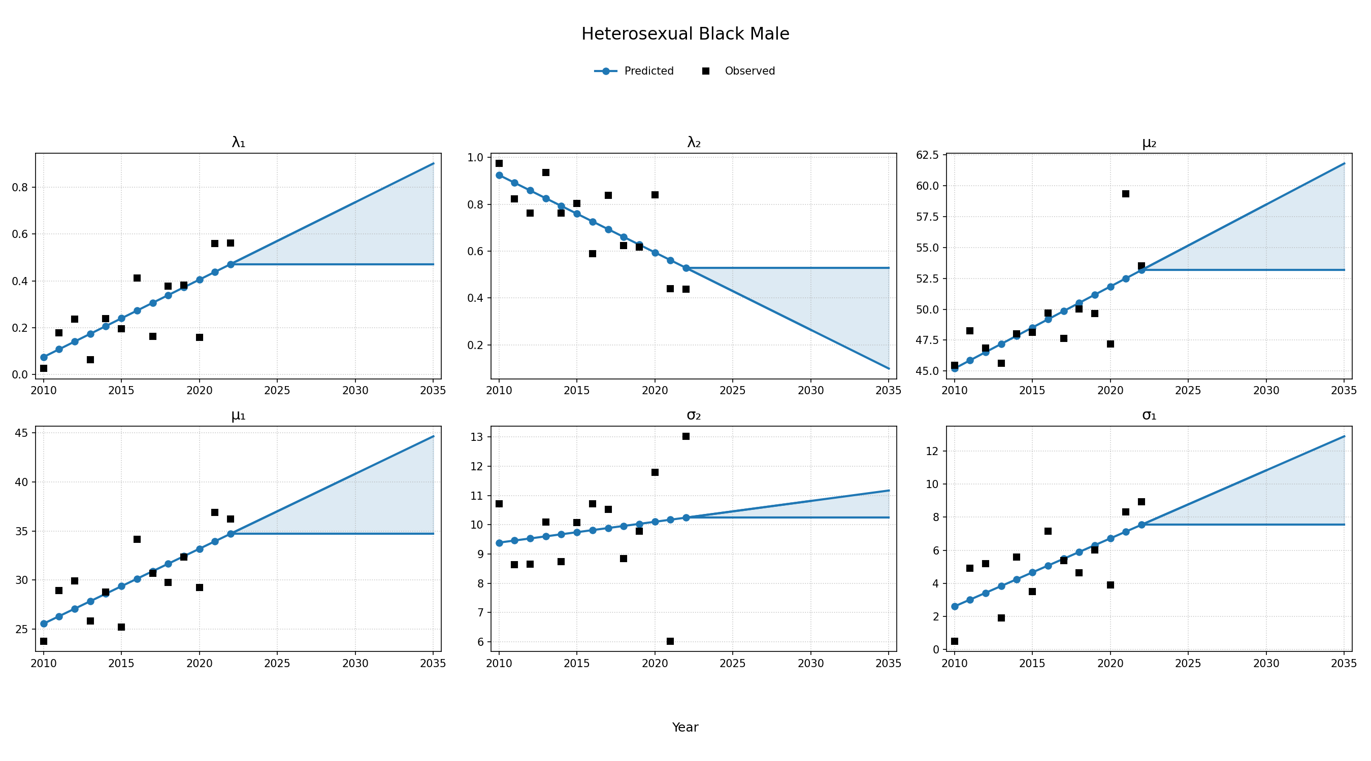
Figure 4c: HET Hispanic Female
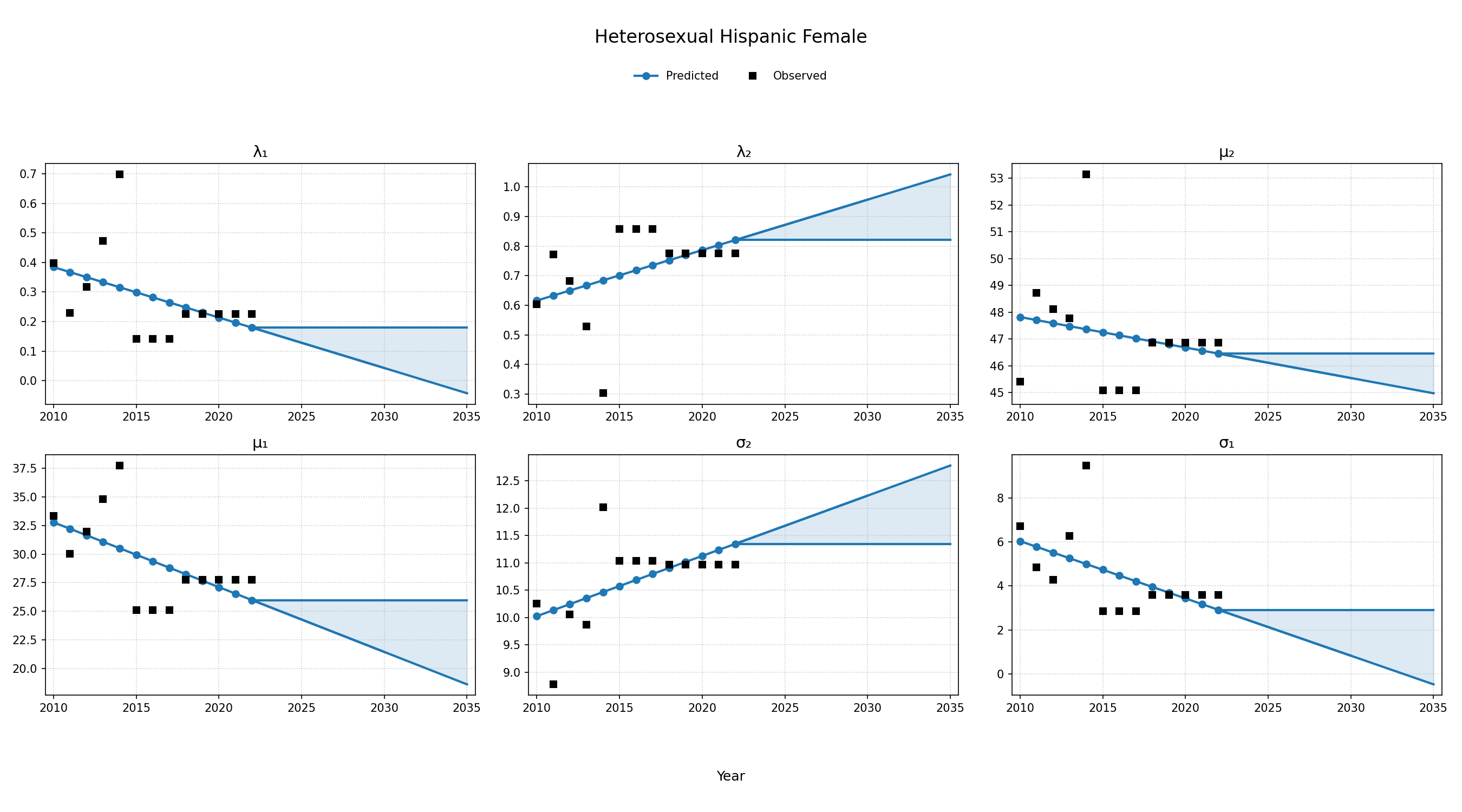
Figure 4d: HET Hispanic Male
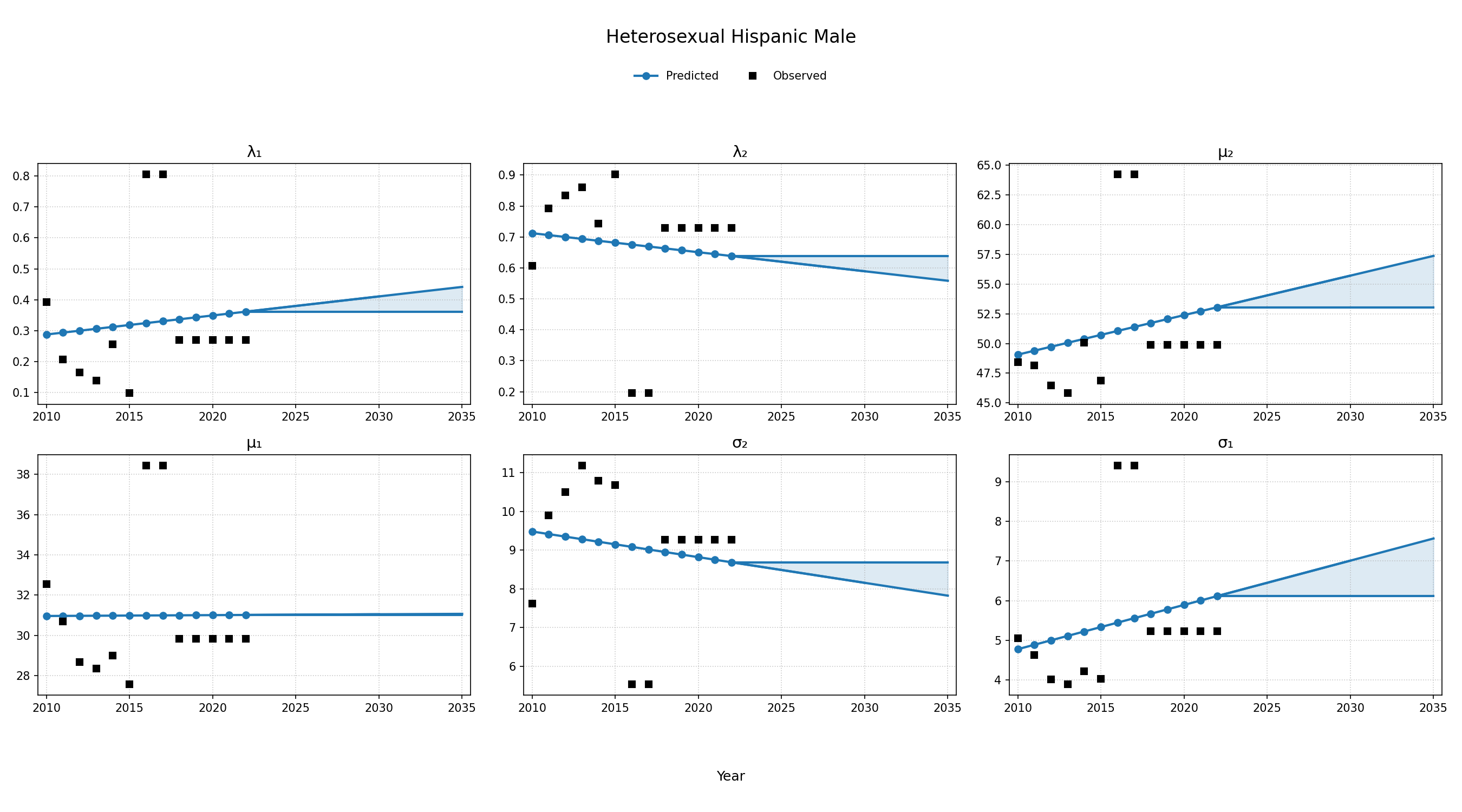
Figure 4e: HET White Female
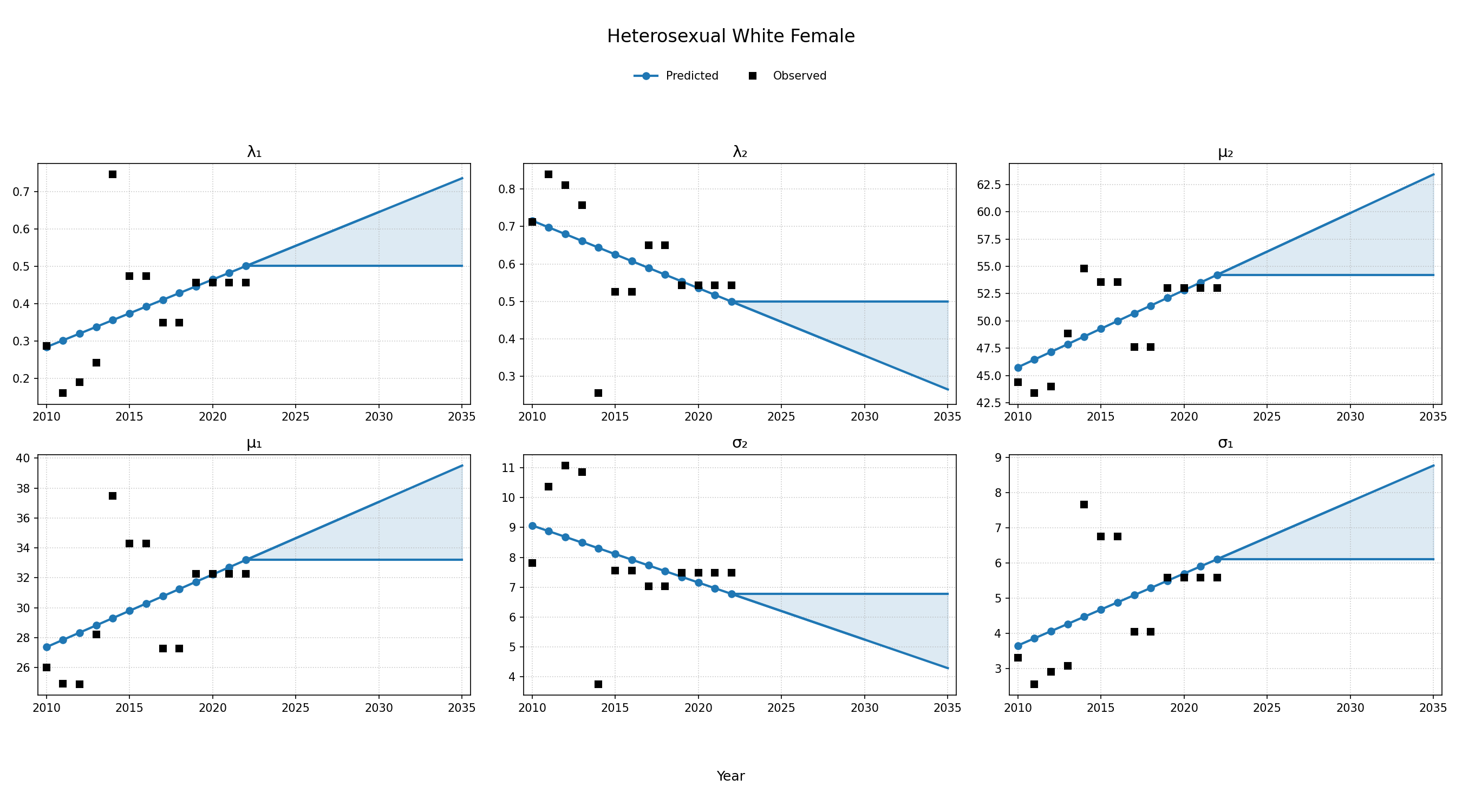
Figure 4f: HET White Male
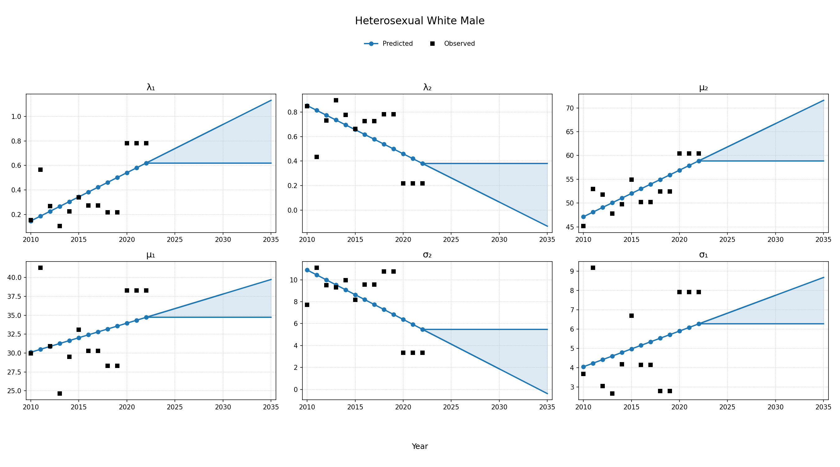
Figure 4g: IDU Black Female
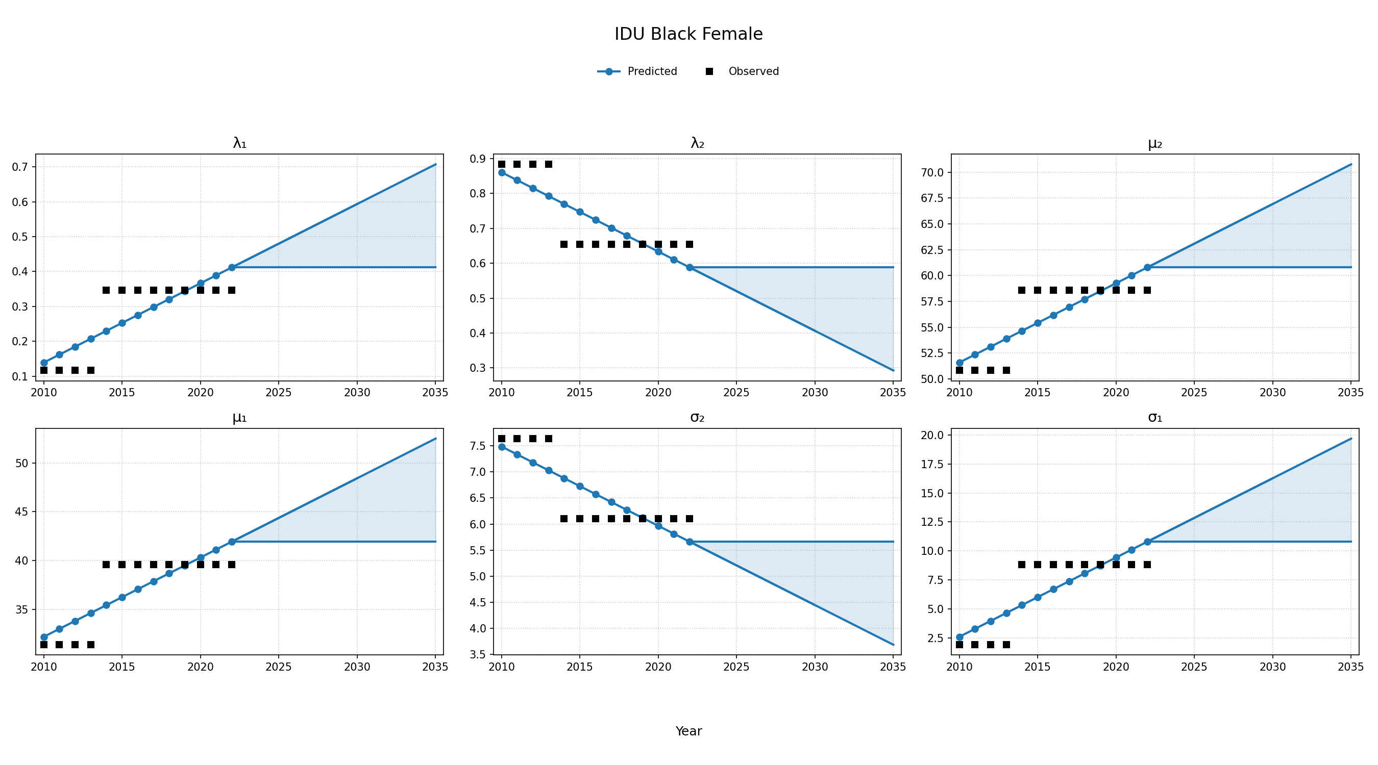
Figure 4h: IDU Black Male
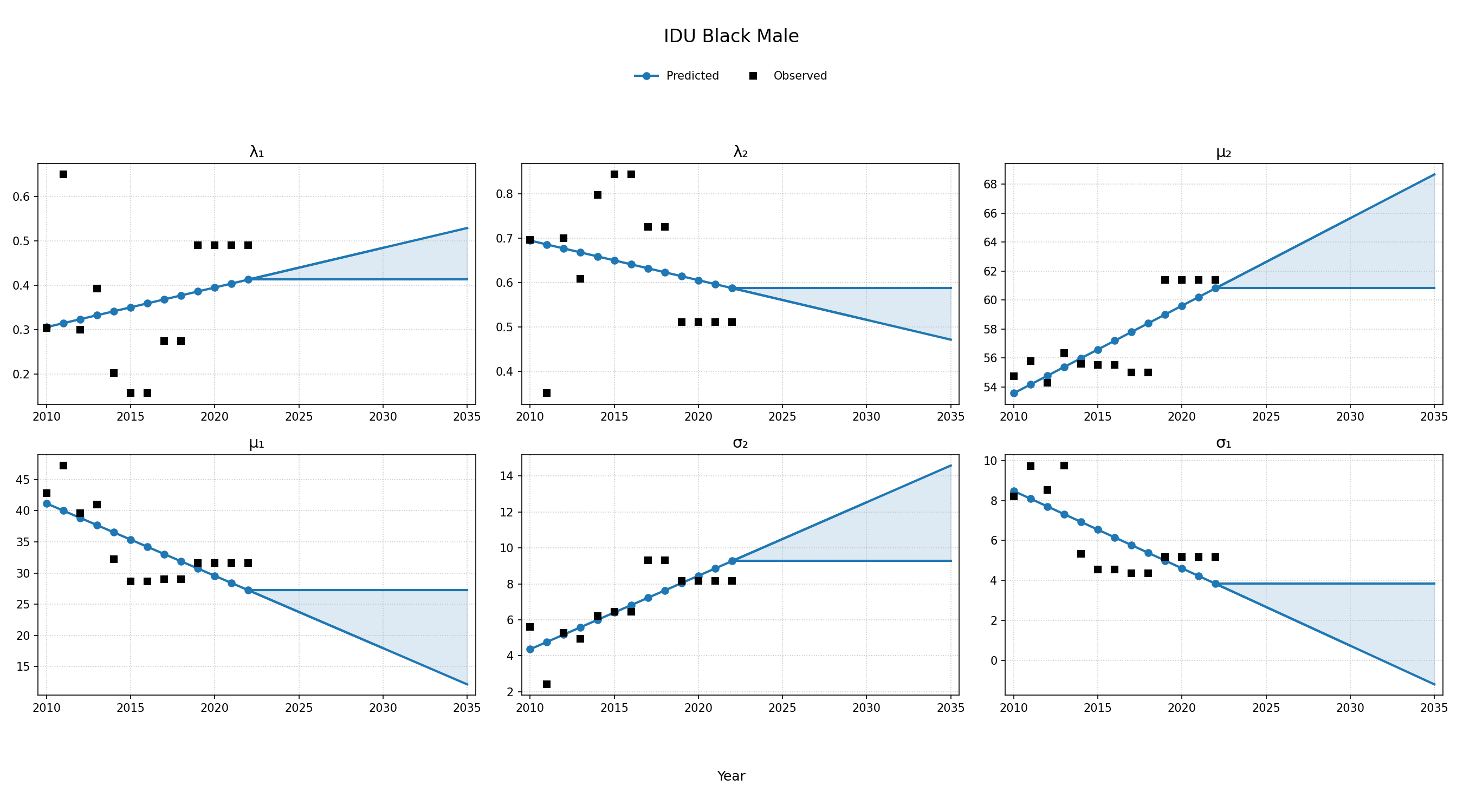
Figure 4i: IDU Hispanic Female
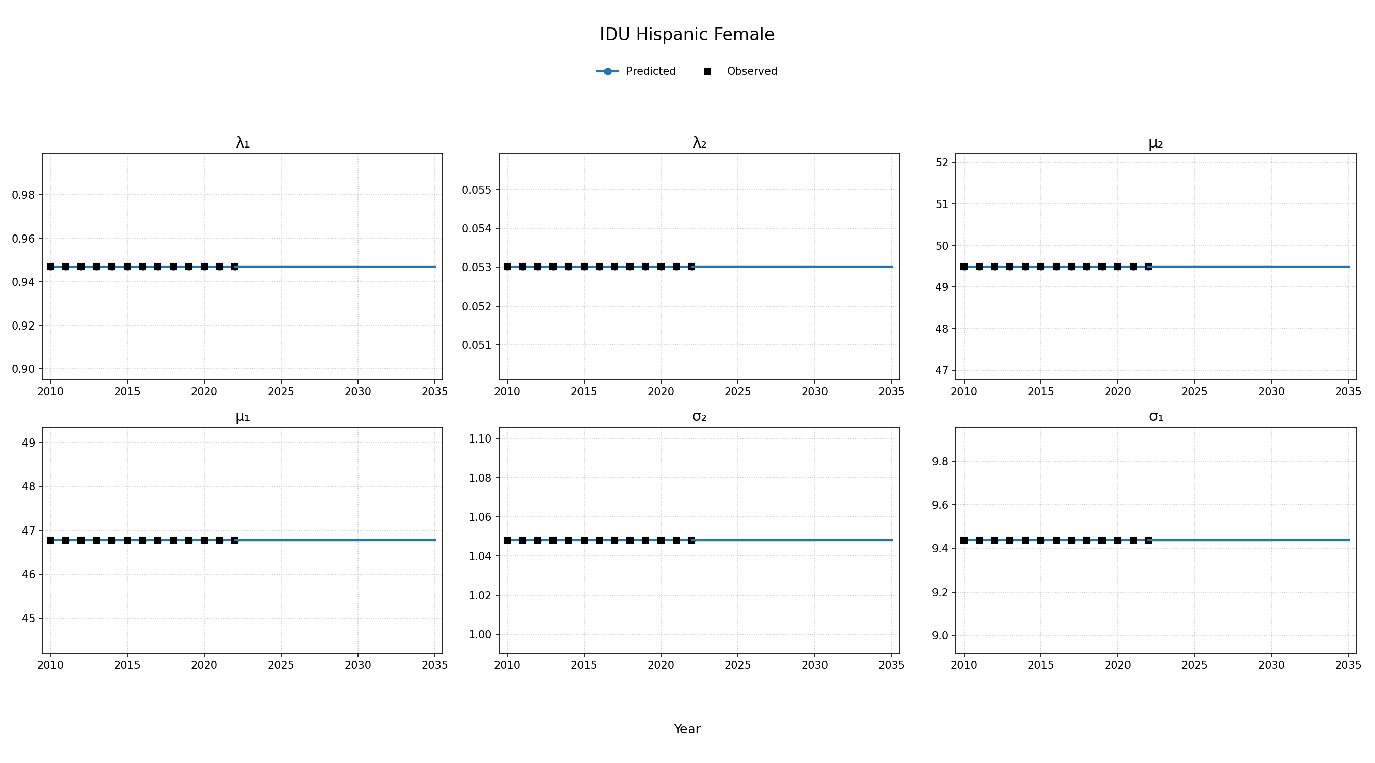
Figure 4j: IDU Hispanic Male
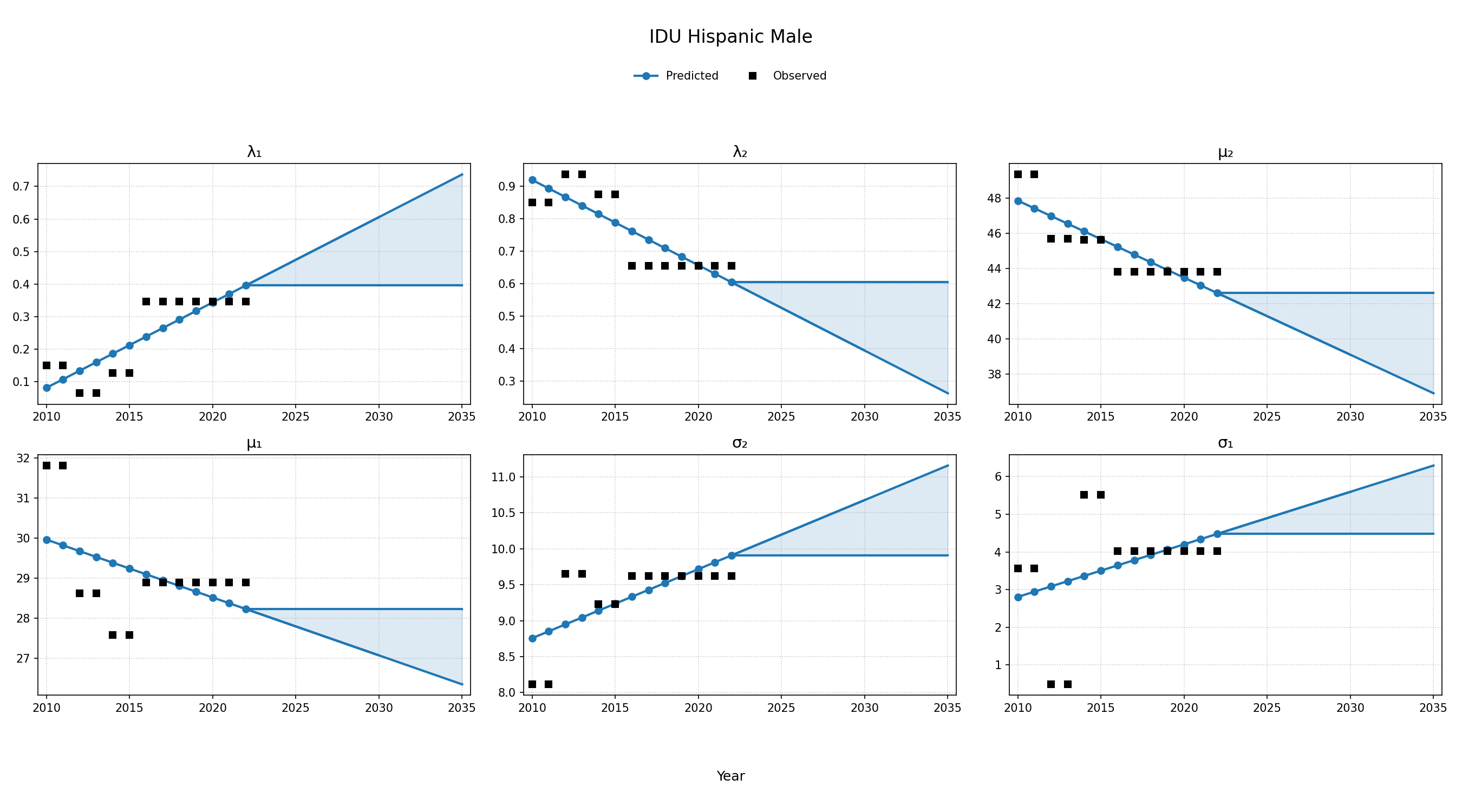
Figure 4k: IDU White Female
Figure 4l: IDU White Male
Figure 4m: Black MSM
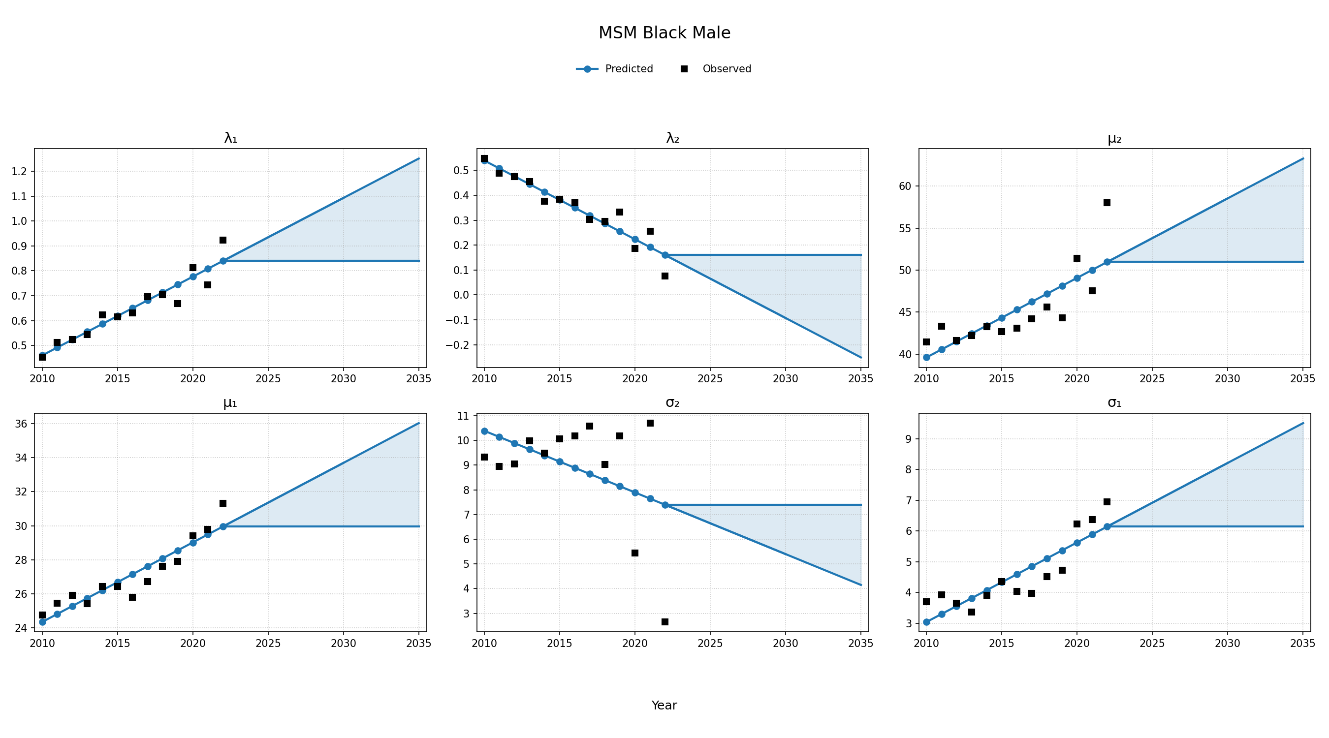
Figure 4n: Hispanic MSM
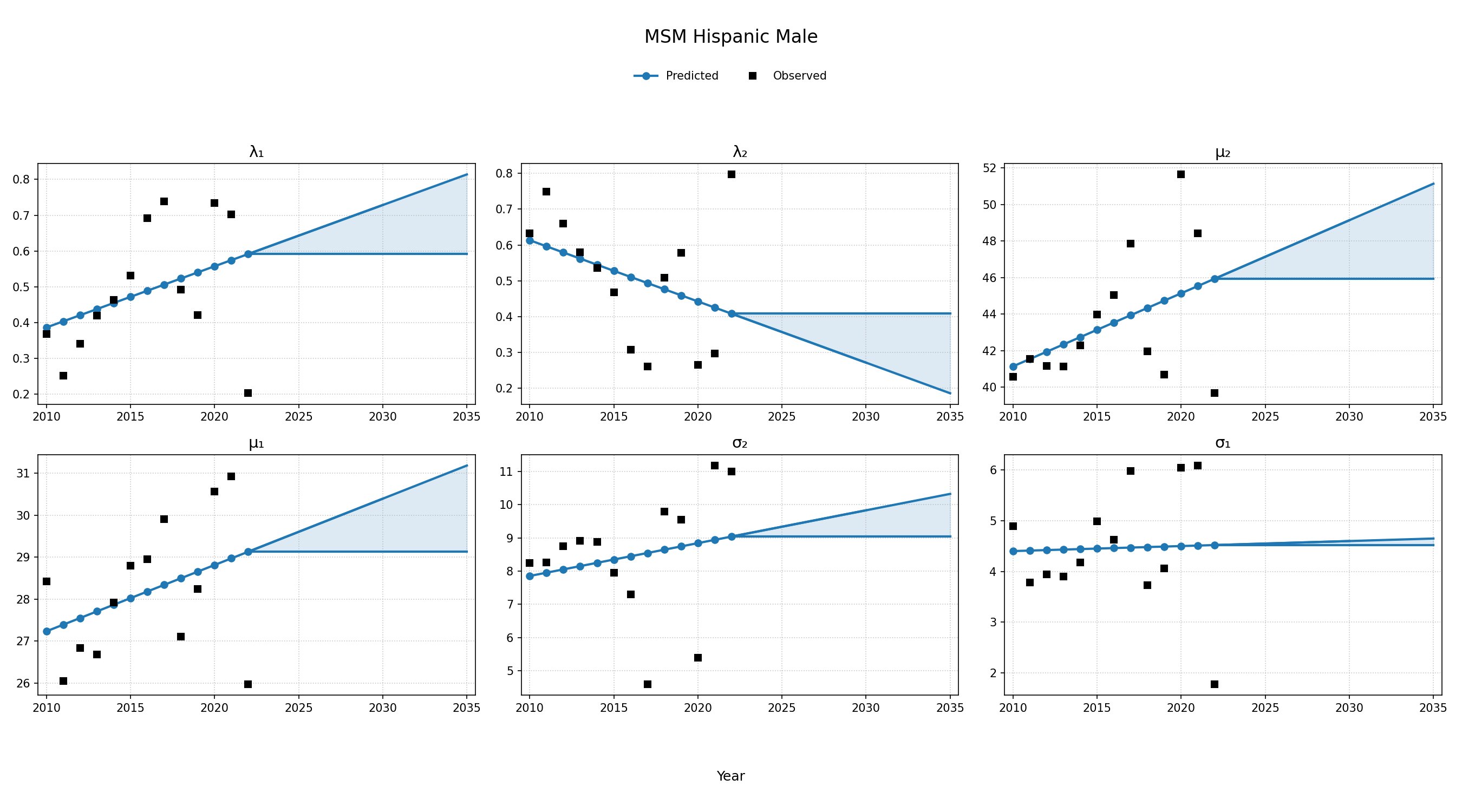
Figure 4o: White MSM
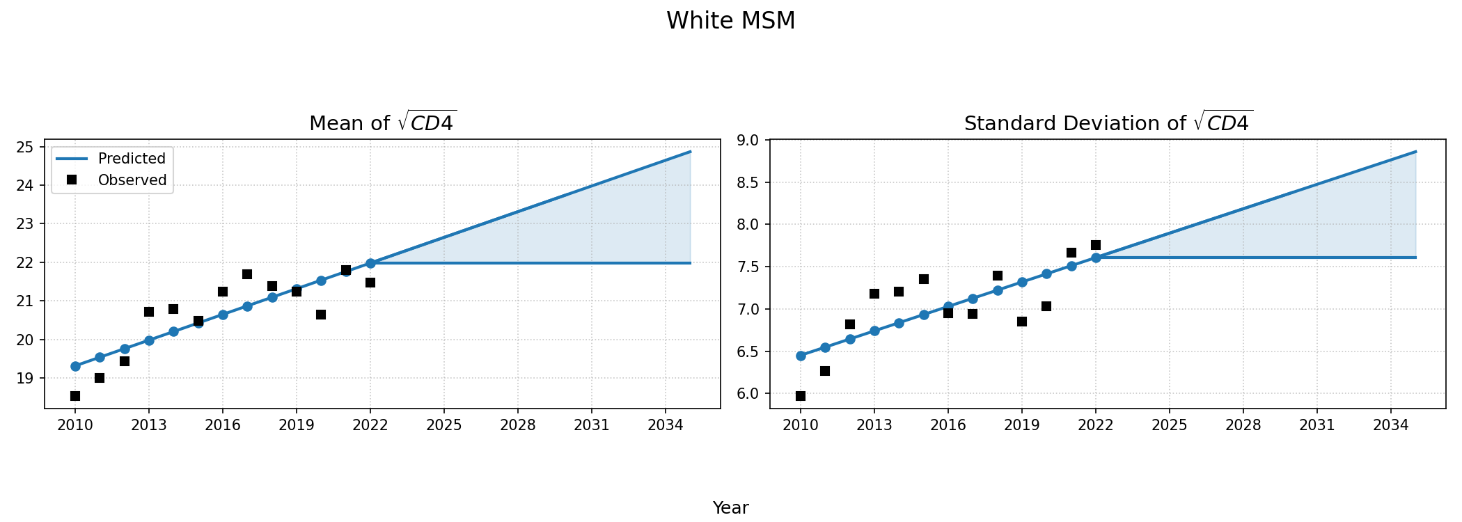
CD4 Count at ART Initiation of ART Initiators</>
Using data from NA-ACCORD, we categorized each sub-populations 8 categories based on ART initiation year (2010 – 2022). A normal distribution was fit to square root of CD4 count values for each sub-group and in each year. Within each sub-population, a linear regression model was applied to describe changes in the normal distribution parameters ($\mu$ mean and $\sigma$ standard deviation) over time, such that:
\[\mu(\mathrm{year}) = \mu_0 + \beta_\mu \cdot \mathrm{year}\]and
\[\sigma(\mathrm{year}) = \sigma_0 + \beta_\sigma \cdot \mathrm{year}\]Some sub-populations had to be collapsed by year in order to generate enough data for the regression according to the following rules:
CD4 Count Data Collapse Rules
Collapse subgroups:
-
All HET men
-
All IDU women
-
All HET women
-
All IDU women
-
All IDU women:
-
2011-2012
-
2014-2016
-
2017-2022
-
-
All IDU men
- 2020-2022
The fits were estimated using the glm function of the stats package in base R. Table 7 presents the value of the fitted coefficients and the trend is shown in Figure 5.
Table 7: ART Initiator Population CD4 Count Coefficients
| group | meanint | meanslp | stdint | stdslp |
|---|---|---|---|---|
| het_hisp_male | -481.12 | 0.25 | -136.09 | 0.07 |
| het_black_male | -481.12 | 0.25 | -136.09 | 0.07 |
| het_white_male | -481.12 | 0.25 | -136.09 | 0.07 |
| idu_black_male | -876.43 | 0.44 | -97.37 | 0.05 |
| idu_hisp_male | -876.43 | 0.44 | -97.37 | 0.05 |
| idu_white_male | -876.43 | 0.44 | -97.37 | 0.05 |
| msm_black_male | -424.13 | 0.22 | -187.66 | 0.10 |
| msm_hisp_male | -459.66 | 0.24 | -38.47 | 0.02 |
| msm_white_male | -427.41 | 0.22 | -187.30 | 0.10 |
| het_black_female | -544.65 | 0.28 | -198.66 | 0.10 |
| het_white_female | -544.65 | 0.28 | -198.66 | 0.10 |
| het_hisp_female | -544.65 | 0.28 | -198.66 | 0.10 |
| idu_black_female | -1121.86 | 0.57 | -59.33 | 0.03 |
| idu_hisp_female | -1121.86 | 0.57 | -59.33 | 0.03 |
| idu_white_female | -1121.86 | 0.57 | -59.33 | 0.03 |
When drawing CD4 values, we truncate the normal distribution at $0$ and $\sqrt{2000}$. Additionally, the predicted values in year 2018 were used as an upper/lower bound to develop a prediction range for future year.
Figure 5a: HET Female
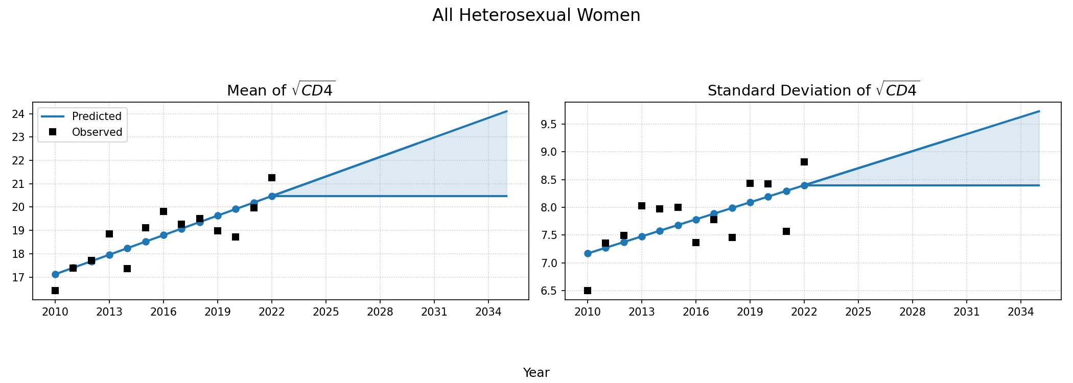
Figure 5b: HET Male
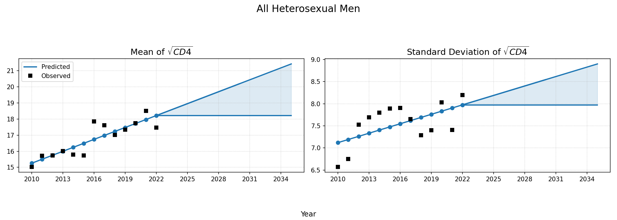
Figure 5c: IDU Female
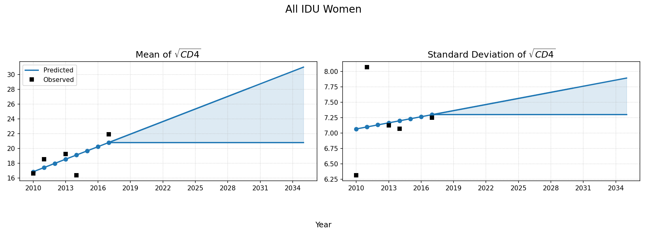
Figure 5d: IDU Male
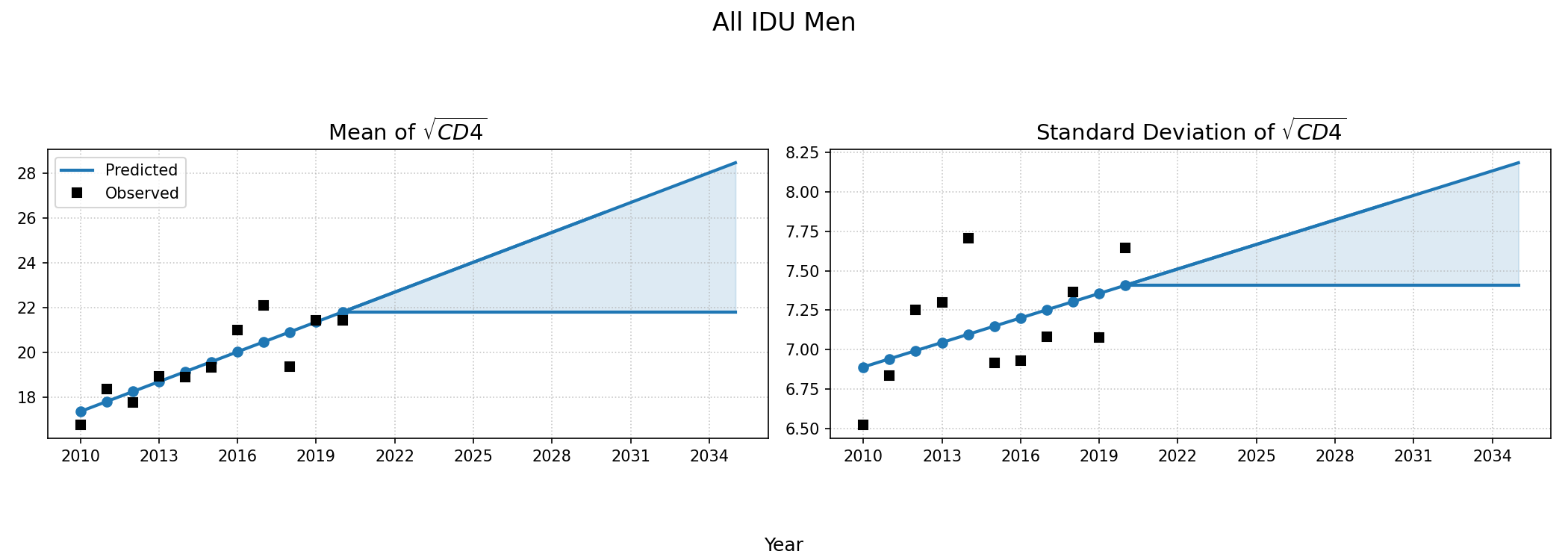
Figure 5e: Black MSM
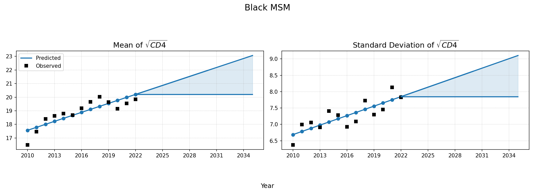
Figure 5e: Hispanic MSM
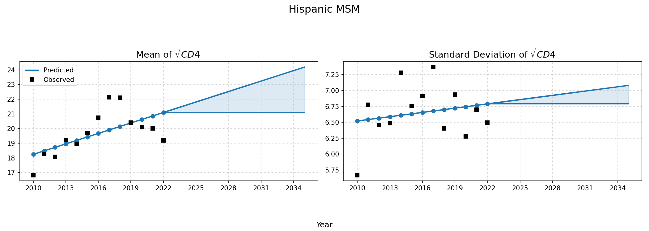
Figure 5e: White MSM
Annual Population Dynamics </>
Disengagement From HIV Care </>
The NA-ACCORD dataset was restricted to the years 2009 – 2022 and each patient was represented by a data point for each year they were alive and under observation in NA-ACCORD. A patient was defined to be disengaged if ≥2 years had elapsed without a CD4 or viral load lab result and the year of disengagement was set to the first year without a lab. Using this data, a logistic regression was used to model the probability of disengagement as a function of calendar year ($\mathrm{year}$), square root of CD4 count at ART initiation (\(\mathrm{sqrt\_init\_cd4}\)), ART initiation period (\(\mathrm{art\_period}\)), and age ($\mathrm{age}$). ART initiation period was coded as a binary variable such that \(\mathrm{art\_period} = 1\) if ART was initiated after 2010 and 0 otherwise. Age is modeled as a restricted quadratic spline with 4 knots. The knots were placed at the 0.05, 0.35, 0.65, and 0.95 quantiles of the $\mathrm{age}$ variable (Table 8). The knot variables are defined such that
\[\mathrm{age}\_1 = \begin{cases} \frac{(\mathrm{age} - k_1)^2 - (\mathrm{age} - k_4)^2}{k_4 - k_1}, & \mathrm{age} \ge k_4\\ \frac{(\mathrm{age} - k_1)^2} {k_4 - k_1}, & k_4 \gt \mathrm{age} \ge k_1\\ 0, & \mathrm{else} \end{cases}\] \[\mathrm{age}\_2 = \begin{cases} \frac{(\mathrm{age} - k_2)^2 - (\mathrm{age} - k_4)^2}{k_4 - k_1}, & \mathrm{age} \ge k_4\\ \frac{(\mathrm{age} - k_2)^2} {k_4 - k_1}, & k_4 \gt \mathrm{age} \ge k_2\\ 0, & \mathrm{else} \end{cases}\] \[\mathrm{age}\_3 = \begin{cases} \frac{(\mathrm{age} - k_3)^2 - (\mathrm{age} - k_4)^2}{k_4 - k_1}, & \mathrm{age} \ge k_4\\ \frac{(\mathrm{age} - k_3)^2} {k_4 - k_1}, & k_4 \gt \mathrm{age} \ge k_3\\ 0, & \mathrm{else} \end{cases}\]Table 8: Disengagement Spline Knot Locations
| subgroup | knot_1 | knot_2 | knot_3 | knot_4 |
|---|---|---|---|---|
| het_black_female | 28 | 42 | 51 | 65 |
| het_black_male | 31 | 47 | 56 | 69 |
| het_hisp_female | 29 | 41 | 50 | 65 |
| het_hisp_male | 30 | 44 | 53 | 69 |
| het_white_female | 28 | 44 | 53 | 67 |
| het_white_male | 32 | 48 | 57 | 71 |
| idu_black_female | 38 | 50 | 57 | 67 |
| idu_black_male | 40 | 55 | 61 | 70 |
| idu_hisp_female | 33 | 46 | 53 | 64 |
| idu_hisp_male | 31 | 47 | 55 | 67 |
| idu_white_female | 31 | 44 | 52 | 63 |
| idu_white_male | 30 | 46 | 54 | 66 |
| msm_black_male | 24 | 35 | 49 | 64 |
| msm_hisp_male | 26 | 38 | 47 | 62 |
| msm_white_male | 29 | 46 | 54 | 68 |
The resulting regression equation is
\[\begin{aligned} \mathrm{logit}(p) = \beta\_0 &+ \beta\_\mathrm{year} \cdot\mathrm{year} + \beta\_\mathrm{sqrt\\init\\cd4} \cdot\mathrm{sqrt\\init\\cd4} + \beta\_\mathrm{art\\period} \cdot \mathrm{art\\period} \\ &+ \beta\_\mathrm{age} \cdot\mathrm{age} + \beta\_\mathrm{age\\1} \cdot\mathrm{age\\1} + \beta\_\mathrm{age\\2} \cdot\mathrm{age\\2} + \beta\_\mathrm{age\\3} \cdot\mathrm{age\\3} \end{aligned}\]where
\[\mathrm{logit}(p) = \log \frac{p}{1 - p}\]is the logit function and $p$ is the probability of disengagement from HIV care.
The coefficients were estimated using a generalized estimating equation (GEE) with a logit link and an exchangeable correlation structure using the geeglm function of the geepack software package for R. The estimated regression coefficients are shown in Table 9 and the covariance matrices is shown in Table 10.
Table 9: Disengagement Coefficient Estimates
| group | intercept | age | _age | __age | ___age | year | sqrtcd4n | haart_period |
|---|---|---|---|---|---|---|---|---|
| het_black_male | 99.84 | -0.01 | -0.01 | -0.08 | 0.15 | -0.05 | 0.00 | 0.20 |
| het_black_female | 96.30 | -0.01 | -0.03 | 0.04 | 0.00 | -0.05 | 0.01 | 0.10 |
| het_hisp_male | 35.60 | -0.01 | -0.03 | 0.04 | 0.01 | -0.02 | 0.02 | -0.02 |
| het_hisp_female | 117.63 | -0.04 | 0.14 | -0.29 | 0.19 | -0.06 | -0.01 | 0.29 |
| het_white_male | 56.28 | -0.03 | 0.03 | -0.16 | 0.14 | -0.03 | 0.01 | 0.10 |
| het_white_female | 74.75 | -0.02 | -0.02 | 0.04 | -0.01 | -0.04 | 0.00 | 0.02 |
| idu_black_male | 87.38 | -0.03 | 0.03 | -0.27 | 0.40 | -0.04 | 0.00 | 0.53 |
| idu_black_female | 67.06 | -0.01 | -0.03 | 0.19 | -0.27 | -0.03 | 0.00 | 0.45 |
| idu_hisp_male | 26.06 | -0.02 | -0.01 | 0.03 | -0.13 | -0.01 | -0.01 | 0.10 |
| idu_hisp_female | -99.03 | -0.02 | 0.03 | -0.29 | 0.37 | 0.05 | -0.01 | -0.48 |
| idu_white_male | 20.63 | 0.01 | -0.05 | 0.05 | -0.16 | -0.01 | 0.01 | 0.14 |
| idu_white_female | 21.77 | 0.01 | -0.11 | 0.32 | -0.22 | -0.01 | 0.01 | -0.32 |
| msm_black_male | 36.98 | 0.07 | -0.22 | 0.25 | -0.03 | -0.02 | 0.01 | 0.07 |
| msm_hisp_male | 15.99 | 0.07 | -0.18 | 0.26 | -0.10 | -0.01 | 0.01 | -0.03 |
| msm_white_male | 31.14 | 0.00 | -0.06 | 0.12 | -0.07 | -0.02 | 0.01 | 0.00 |
Table 10 Variance and Covariance
| group | varname | intercept | age | _age | __age | ___age | year | sqrtcd4n | haart_period |
|---|---|---|---|---|---|---|---|---|---|
| het_black_female | intercept | 185.271075 | 0.007836522 | -0.00112997 | 0.019492126 | -0.026039776 | -0.092245869 | 0.002741405 | 0.284554514 |
| het_black_female | age | 0.007836522 | 1.25E-04 | -2.73E-04 | 5.23E-04 | -3.26E-04 | -5.78E-06 | 3.79E-06 | 3.04E-05 |
| het_black_female | _age | -0.00112997 | -2.73E-04 | 7.05E-04 | -0.001582584 | 0.001197041 | 4.43E-06 | -3.21E-06 | 1.99E-05 |
| het_black_female | __age | 0.019492126 | 5.23E-04 | -0.001582584 | 0.004277036 | -0.004021257 | -1.68E-05 | -1.04E-06 | -7.38E-05 |
| het_black_female | ___age | -0.026039776 | -3.26E-04 | 0.001197041 | -0.004021257 | 0.004779601 | 1.71E-05 | 4.76E-06 | 7.99E-05 |
| het_black_female | year | -0.092245869 | -5.78E-06 | 4.43E-06 | -1.68E-05 | 1.71E-05 | 4.60E-05 | -1.53E-06 | -1.42E-04 |
| het_black_female | sqrtcd4n | 0.002741405 | 3.79E-06 | -3.21E-06 | -1.04E-06 | 4.76E-06 | -1.53E-06 | 1.31E-05 | -3.72E-05 |
| het_black_female | haart_period | 0.284554514 | 3.04E-05 | 1.99E-05 | -7.38E-05 | 7.99E-05 | -1.42E-04 | -3.72E-05 | 0.003311122 |
| het_black_male | intercept | 219.8332737 | -0.003800992 | 0.013663238 | 0.042994107 | -0.101107108 | -0.109208728 | -0.001681469 | 0.356953658 |
| het_black_male | age | -0.003800992 | 1.12E-04 | -2.22E-04 | 4.68E-04 | -3.37E-04 | 2.45E-08 | 1.79E-06 | 7.80E-05 |
| het_black_male | _age | 0.013663238 | -2.22E-04 | 5.17E-04 | -0.001297461 | 0.001117953 | -3.29E-06 | -2.81E-06 | -6.36E-05 |
| het_black_male | __age | 0.042994107 | 4.68E-04 | -0.001297461 | 0.004185503 | -0.004662877 | -2.84E-05 | 1.23E-07 | 2.46E-04 |
| het_black_male | ___age | -0.101107108 | -3.37E-04 | 0.001117953 | -0.004662877 | 0.006636827 | 5.51E-05 | 3.07E-06 | -3.14E-04 |
| het_black_male | year | -0.109208728 | 2.45E-08 | -3.29E-06 | -2.84E-05 | 5.51E-05 | 5.43E-05 | 7.17E-07 | -1.79E-04 |
| het_black_male | sqrtcd4n | -0.001681469 | 1.79E-06 | -2.81E-06 | 1.23E-07 | 3.07E-06 | 7.17E-07 | 1.33E-05 | -3.70E-05 |
| het_black_male | haart_period | 0.356953658 | 7.80E-05 | -6.36E-05 | 2.46E-04 | -3.14E-04 | -1.79E-04 | -3.70E-05 | 0.003917841 |
| het_hisp_female | intercept | 845.8712519 | 0.022060761 | 0.029632616 | -0.145485142 | 0.261762632 | -0.42085395 | 0.001447187 | 0.853297485 |
| het_hisp_female | age | 0.022060761 | 7.46E-04 | -0.001756704 | 0.002917353 | -0.001424294 | -2.24E-05 | 1.27E-05 | 1.27E-04 |
| het_hisp_female | _age | 0.029632616 | -0.001756704 | 0.004799058 | -0.009097784 | 0.005529795 | 1.09E-05 | -7.96E-06 | 1.16E-04 |
| het_hisp_female | __age | -0.145485142 | 0.002917353 | -0.009097784 | 0.019808449 | -0.014881799 | 3.12E-05 | -7.77E-06 | -8.65E-04 |
| het_hisp_female | ___age | 0.261762632 | -0.001424294 | 0.005529795 | -0.014881799 | 0.014748728 | -1.11E-04 | 1.70E-05 | 0.001118864 |
| het_hisp_female | year | -0.42085395 | -2.24E-05 | 1.09E-05 | 3.12E-05 | -1.11E-04 | 2.10E-04 | -1.33E-06 | -4.28E-04 |
| het_hisp_female | sqrtcd4n | 0.001447187 | 1.27E-05 | -7.96E-06 | -7.77E-06 | 1.70E-05 | -1.33E-06 | 4.83E-05 | -5.55E-05 |
| het_hisp_female | haart_period | 0.853297485 | 1.27E-04 | 1.16E-04 | -8.65E-04 | 0.001118864 | -4.28E-04 | -5.55E-05 | 0.011886905 |
| het_hisp_male | intercept | 740.3173022 | 0.02787669 | 0.001286347 | 0.132014325 | -0.262730952 | -0.368474736 | -0.007852919 | 1.049815354 |
| het_hisp_male | age | 0.02787669 | 4.03E-04 | -9.26E-04 | 0.001743292 | -0.001019167 | -2.03E-05 | 7.22E-06 | 1.63E-04 |
| het_hisp_male | _age | 0.001286347 | -9.26E-04 | 0.002492909 | -0.005458677 | 0.003861525 | 1.35E-05 | -2.05E-05 | -2.97E-05 |
| het_hisp_male | __age | 0.132014325 | 0.001743292 | -0.005458677 | 0.014447999 | -0.01283614 | -9.13E-05 | 3.62E-05 | -2.28E-04 |
| het_hisp_male | ___age | -0.262730952 | -0.001019167 | 0.003861525 | -0.01283614 | 0.014420576 | 1.45E-04 | -2.98E-05 | 3.87E-04 |
| het_hisp_male | year | -0.368474736 | -2.03E-05 | 1.35E-05 | -9.13E-05 | 1.45E-04 | 1.84E-04 | 3.52E-06 | -5.26E-04 |
| het_hisp_male | sqrtcd4n | -0.007852919 | 7.22E-06 | -2.05E-05 | 3.62E-05 | -2.98E-05 | 3.52E-06 | 4.34E-05 | -1.09E-04 |
| het_hisp_male | haart_period | 1.049815354 | 1.63E-04 | -2.97E-05 | -2.28E-04 | 3.87E-04 | -0.000525765 | -0.000109101 | 0.011389478 |
| het_white_female | intercept | 654.3233874 | 0.007762047 | 0.049619856 | -0.058638006 | -3.33E-04 | -0.325455559 | 0.001299009 | 1.155309545 |
| het_white_female | age | 0.007762047 | 4.00E-04 | -8.04E-04 | 0.001663796 | -0.001135938 | -9.99E-06 | 1.25E-05 | 2.74E-04 |
| het_white_female | _age | 0.049619856 | -8.04E-04 | 0.001883184 | -0.004589327 | 0.003762243 | -1.30E-05 | -8.77E-06 | -1.48E-04 |
| het_white_female | __age | -0.058638006 | 0.001663796 | -0.004589327 | 0.014129341 | -0.014897406 | 6.13E-06 | -4.09E-06 | -1.41E-04 |
| het_white_female | ___age | -3.33E-04 | -0.001135938 | 0.003762243 | -0.014897406 | 0.020073382 | 1.51E-05 | 1.43E-05 | 5.94E-04 |
| het_white_female | year | -0.325455559 | -9.99E-06 | -1.30E-05 | 6.13E-06 | 1.51E-05 | 1.62E-04 | -1.26E-06 | -5.80E-04 |
| het_white_female | sqrtcd4n | 0.001299009 | 1.25E-05 | -8.77E-06 | -4.09E-06 | 1.43E-05 | -1.26E-06 | 4.62E-05 | -1.27E-04 |
| het_white_female | haart_period | 1.155309544 | 2.74E-04 | -1.48E-04 | -1.41E-04 | 5.94E-04 | -5.80E-04 | -1.27E-04 | 0.012967097 |
| het_white_male | intercept | 713.6727774 | 0.013555743 | 0.007645773 | 0.146567513 | -0.328952296 | -0.354955502 | 0.003842253 | 1.128869518 |
| het_white_male | age | 0.013555743 | 3.33E-04 | -7.00E-04 | 0.001527218 | -0.001130891 | -1.24E-05 | 1.31E-05 | 3.89E-04 |
| het_white_male | _age | 0.007645773 | -7.00E-04 | 0.001780393 | -0.004664282 | 0.004123648 | 7.33E-06 | -1.30E-05 | -2.41E-04 |
| het_white_male | __age | 0.146567513 | 0.001527218 | -0.004664282 | 0.015480648 | -0.017296718 | -9.58E-05 | 2.27E-05 | -2.63E-04 |
| het_white_male | ___age | -0.328952296 | -0.001130891 | 0.004123648 | -0.017296718 | 0.024403704 | 1.80E-04 | -2.84E-05 | 6.61E-04 |
| het_white_male | year | -0.354955502 | -1.24E-05 | 7.33E-06 | -9.58E-05 | 1.80E-04 | 1.77E-04 | -2.55E-06 | -5.70E-04 |
| het_white_male | sqrtcd4n | 0.003842253 | 1.31E-05 | -1.30E-05 | 2.27E-05 | -2.84E-05 | -2.55E-06 | 5.09E-05 | -9.00E-05 |
| het_white_male | haart_period | 1.128869518 | 3.89E-04 | -2.41E-04 | -2.63E-04 | 6.61E-04 | -5.70E-04 | -9.00E-05 | 0.013566181 |
| idu_black_female | intercept | 2096.233051 | -0.098940686 | 0.5938993 | -1.551873166 | 1.986007683 | -1.040674113 | 0.030376871 | 2.480864945 |
| idu_black_female | age | -0.098940686 | 0.001147934 | -0.002467392 | 0.005186504 | -0.003692398 | 2.69E-05 | 2.03E-05 | 0.001090253 |
| idu_black_female | _age | 0.5938993 | -0.002467392 | 0.006638436 | -0.016980648 | 0.014955653 | -2.50E-04 | -2.83E-05 | -9.12E-04 |
| idu_black_female | __age | -1.551873166 | 0.005186504 | -0.016980648 | 0.053988459 | -0.060338806 | 6.79E-04 | 3.56E-05 | -2.52E-04 |
| idu_black_female | ___age | 1.986007683 | -0.003692398 | 0.014955653 | -0.060338806 | 0.088340606 | -9.24E-04 | 6.37E-05 | 0.001691034 |
| idu_black_female | year | -1.040674113 | 2.69E-05 | -2.50E-04 | 6.79E-04 | -9.24E-04 | 5.17E-04 | -1.65E-05 | -0.001256089 |
| idu_black_female | sqrtcd4n | 0.030376871 | 2.03E-05 | -2.83E-05 | 3.56E-05 | 6.37E-05 | -1.65E-05 | 1.28E-04 | -5.78E-04 |
| idu_black_female | haart_period | 2.480864945 | 0.001090253 | -9.12E-04 | -2.52E-04 | 0.001691034 | -0.001256089 | -5.78E-04 | 0.042875289 |
| idu_black_male | intercept | 897.2968632 | -0.064000065 | 0.143588783 | 0.270373501 | -0.531521829 | -0.444789038 | -5.59E-05 | 1.439990739 |
| idu_black_male | age | -0.064000065 | 1.71E-04 | -3.43E-04 | 0.001033269 | -9.96E-04 | 2.83E-05 | 8.05E-06 | 3.13E-04 |
| idu_black_male | _age | 0.143588783 | -3.43E-04 | 9.43E-04 | -0.003807912 | 0.004366243 | -6.50E-05 | -2.31E-05 | -7.49E-05 |
| idu_black_male | __age | 0.270373501 | 0.001033269 | -0.003807912 | 0.02382312 | -0.035678079 | -1.52E-04 | 7.47E-05 | 6.12E-04 |
| idu_black_male | ___age | -0.531521829 | -9.96E-04 | 0.004366243 | -0.035678079 | 0.06529744 | 2.81E-04 | -4.42E-05 | -0.001102303 |
| idu_black_male | year | -0.444789038 | 2.83E-05 | -6.50E-05 | -1.52E-04 | 2.81E-04 | 2.21E-04 | -4.16E-07 | -7.24E-04 |
| idu_black_male | sqrtcd4n | -5.59E-05 | 8.05E-06 | -2.31E-05 | 7.47E-05 | -4.42E-05 | -4.16E-07 | 4.32E-05 | -2.02E-04 |
| idu_black_male | haart_period | 1.439990739 | 3.13E-04 | -7.49E-05 | 6.12E-04 | -0.001102303 | -7.24E-04 | -2.02E-04 | 0.016495406 |
| idu_hisp_female | intercept | 10303.62837 | 2.93148134 | -3.634019384 | 3.924816885 | 1.824005448 | -5.179937022 | 0.237727822 | 18.66993272 |
| idu_hisp_female | age | 2.93148134 | 0.006181422 | -0.011318588 | 0.021592835 | -0.011866228 | -0.001566012 | 1.39E-05 | 0.006559636 |
| idu_hisp_female | _age | -3.634019385 | -0.011318588 | 0.023657791 | -0.052703708 | 0.035993078 | 0.001999176 | 1.98E-05 | -0.00856183 |
| idu_hisp_female | __age | 3.924816885 | 0.021592835 | -0.052703708 | 0.148621693 | -0.133089097 | -0.002309008 | 5.12E-05 | 0.010279091 |
| idu_hisp_female | ___age | 1.824005447 | -0.011866228 | 0.035993078 | -0.133089097 | 0.153228848 | -7.18E-04 | -1.01E-04 | 0.003898479 |
| idu_hisp_female | year | -5.179937022 | -0.001566012 | 0.001999176 | -0.002309008 | -7.18E-04 | 0.002605734 | -1.21E-04 | -0.009415165 |
| idu_hisp_female | sqrtcd4n | 0.237727822 | 1.39E-05 | 1.98E-05 | 5.12E-05 | -1.01E-04 | -1.21E-04 | 3.11E-04 | -1.53E-04 |
| idu_hisp_female | haart_period | 18.66993272 | 0.006559636 | -0.00856183 | 0.010279091 | 0.003898479 | -0.009415165 | -1.53E-04 | 0.157836669 |
| idu_hisp_male | intercept | 1050.706389 | 0.003443364 | -0.030011124 | 0.422739961 | -0.447761722 | -0.522622756 | 0.035896928 | 1.713012712 |
| idu_hisp_male | age | 0.003443364 | 5.68E-04 | -0.001056991 | 0.002380021 | -0.001854311 | -1.13E-05 | 2.05E-05 | 5.80E-04 |
| idu_hisp_male | _age | -0.030011124 | -0.001056991 | 0.002297511 | -0.006236331 | 0.005830005 | 3.20E-05 | -3.90E-05 | -5.94E-04 |
| idu_hisp_male | __age | 0.422739961 | 0.002380021 | -0.006236331 | 0.023031557 | -0.02884396 | -2.47E-04 | 8.60E-05 | 0.001499508 |
| idu_hisp_male | ___age | -0.447761722 | -0.001854311 | 0.005830005 | -0.02884396 | 0.047628639 | 2.50E-04 | -1.87E-05 | -0.001678896 |
| idu_hisp_male | year | -0.522622756 | -1.13E-05 | 3.20E-05 | -2.47E-04 | 2.50E-04 | 2.60E-04 | -1.87E-05 | -8.63E-04 |
| idu_hisp_male | sqrtcd4n | 0.035896928 | 2.05E-05 | -3.90E-05 | 8.60E-05 | -1.87E-05 | -1.87E-05 | 7.57E-05 | -2.59E-04 |
| idu_hisp_male | haart_period | 1.713012712 | 5.80E-04 | -5.94E-04 | 0.001499508 | -0.001678896 | -8.63E-04 | -2.59E-04 | 0.021125133 |
| idu_white_female | intercept | 2499.803078 | 0.212015328 | -0.185026074 | 0.618285671 | -0.57323304 | -1.247012381 | 0.079762419 | 4.96571129 |
| idu_white_female | age | 0.212015328 | 0.0016972 | -0.003363702 | 0.006660172 | -0.004656974 | -1.33E-04 | 2.73E-05 | 0.001005909 |
| idu_white_female | _age | -0.185026074 | -0.003363702 | 0.008079744 | -0.019509631 | 0.017087133 | 1.45E-04 | -3.05E-05 | -5.74E-04 |
| idu_white_female | __age | 0.618285671 | 0.006660172 | -0.019509631 | 0.059563343 | -0.066647369 | -4.09E-04 | 2.76E-05 | 7.08E-04 |
| idu_white_female | ___age | -0.57323304 | -0.004656974 | 0.017087133 | -0.066647369 | 0.093905921 | 3.52E-04 | 1.55E-04 | -0.003054944 |
| idu_white_female | year | -1.247012382 | -1.33E-04 | 1.45E-04 | -4.09E-04 | 3.52E-04 | 6.23E-04 | -4.16E-05 | -0.002491198 |
| idu_white_female | sqrtcd4n | 0.079762419 | 2.73E-05 | -3.05E-05 | 2.76E-05 | 1.55E-04 | -4.16E-05 | 1.70E-04 | -6.73E-05 |
| idu_white_female | haart_period | 4.965711291 | 0.001005909 | -5.74E-04 | 7.08E-04 | -0.003054944 | -0.002491198 | -6.73E-05 | 0.050911691 |
| idu_white_male | intercept | 422.4689226 | -0.011817005 | 0.062160748 | -0.121173229 | 0.134891904 | -0.209810006 | -0.004497995 | 0.815994573 |
| idu_white_male | age | -0.011817005 | 2.71E-04 | -5.13E-04 | 0.001187788 | -9.85E-04 | 1.51E-06 | 3.04E-06 | 1.04E-04 |
| idu_white_male | _age | 0.062160748 | -5.13E-04 | 0.0011508 | -0.003239405 | 0.003233182 | -2.31E-05 | 3.83E-06 | 1.95E-04 |
| idu_white_male | __age | -0.12117323 | 0.001187788 | -0.003239405 | 0.012378766 | -0.016523074 | 4.33E-05 | -3.78E-05 | -0.001007757 |
| idu_white_male | ___age | 0.134891904 | -9.85E-04 | 0.003233182 | -0.016523074 | 0.029717938 | -5.38E-05 | 5.39E-05 | 0.001306192 |
| idu_white_male | year | -0.209810006 | 1.51E-06 | -2.31E-05 | 4.33E-05 | -5.38E-05 | 1.04E-04 | 1.87E-06 | -4.08E-04 |
| idu_white_male | sqrtcd4n | -0.004497995 | 3.04E-06 | 3.83E-06 | -3.78E-05 | 5.39E-05 | 1.87E-06 | 3.63E-05 | -1.59E-04 |
| idu_white_male | haart_period | 0.815994573 | 1.04E-04 | 1.95E-04 | -0.001007757 | 0.001306192 | -4.08E-04 | -1.59E-04 | 0.010028371 |
| msm_black_male | intercept | 109.1186038 | 0.01504293 | -0.029173896 | 0.041740205 | -0.003210434 | -0.054442697 | 0.001064732 | 0.220413383 |
| msm_black_male | age | 0.01504293 | 1.41E-04 | -3.71E-04 | 5.10E-04 | -2.09E-04 | -9.31E-06 | 2.00E-06 | 2.51E-05 |
| msm_black_male | _age | -0.029173896 | -3.71E-04 | 0.001100476 | -0.001655193 | 8.79E-04 | 1.91E-05 | -3.26E-06 | 7.21E-05 |
| msm_black_male | __age | 0.041740205 | 5.10E-04 | -0.001655193 | 0.002699339 | -0.001794198 | -2.70E-05 | 3.76E-06 | -1.37E-04 |
| msm_black_male | ___age | -0.003210434 | -2.09E-04 | 8.79E-04 | -0.001794198 | 0.002044894 | 4.06E-06 | -2.35E-06 | 9.67E-05 |
| msm_black_male | year | -0.054442697 | -9.31E-06 | 1.91E-05 | -2.70E-05 | 4.06E-06 | 2.72E-05 | -6.14E-07 | -1.10E-04 |
| msm_black_male | sqrtcd4n | 0.001064732 | 2.00E-06 | -3.26E-06 | 3.76E-06 | -2.35E-06 | -6.14E-07 | 7.36E-06 | -2.46E-05 |
| msm_black_male | haart_period | 0.220413383 | 2.51E-05 | 7.21E-05 | -1.37E-04 | 9.67E-05 | -1.10E-04 | -2.46E-05 | 0.002257966 |
| msm_hisp_male | intercept | 184.0856325 | 0.014529451 | -0.018705699 | 0.046544573 | -0.028929336 | -0.09174528 | 0.004540654 | 0.339868118 |
| msm_hisp_male | age | 0.014529451 | 2.17E-04 | -5.01E-04 | 8.47E-04 | -4.47E-04 | -1.03E-05 | 1.18E-06 | 1.01E-04 |
| msm_hisp_male | _age | -0.018705699 | -5.01E-04 | 0.001321852 | -0.002543229 | 0.001647847 | 1.61E-05 | 1.68E-06 | -7.27E-05 |
| msm_hisp_male | __age | 0.046544573 | 8.47E-04 | -0.002543229 | 0.005693712 | -0.004611725 | -3.42E-05 | -7.16E-06 | 7.69E-05 |
| msm_hisp_male | ___age | -0.028929336 | -4.47E-04 | 0.001647847 | -0.004611725 | 0.004961619 | 2.00E-05 | 5.93E-06 | -1.19E-05 |
| msm_hisp_male | year | -0.09174528 | -1.03E-05 | 1.61E-05 | -3.42E-05 | 2.00E-05 | 4.58E-05 | -2.40E-06 | -1.71E-04 |
| msm_hisp_male | sqrtcd4n | 0.004540654 | 1.18E-06 | 1.68E-06 | -7.16E-06 | 5.93E-06 | -2.40E-06 | 1.49E-05 | -4.99E-05 |
| msm_hisp_male | haart_period | 0.339868118 | 1.01E-04 | -7.27E-05 | 7.69E-05 | -1.19E-05 | -1.71E-04 | -4.99E-05 | 0.003509684 |
| msm_white_male | intercept | 61.52477965 | 0.00219027 | -0.001110188 | 0.023805685 | -0.034730747 | -0.030621775 | 5.32E-04 | 0.109100492 |
| msm_white_male | age | 0.00219027 | 3.78E-05 | -7.32E-05 | 1.72E-04 | -1.29E-04 | -1.69E-06 | 6.89E-07 | 2.70E-05 |
| msm_white_male | _age | -0.001110188 | -7.32E-05 | 1.64E-04 | -4.53E-04 | 3.93E-04 | 1.65E-06 | -6.49E-07 | -9.62E-06 |
| msm_white_male | __age | 0.023805685 | 1.72E-04 | -4.53E-04 | 0.001640293 | -0.001811147 | -1.43E-05 | 1.26E-06 | 1.22E-05 |
| msm_white_male | ___age | -0.034730747 | -1.29E-04 | 3.93E-04 | -0.001811147 | 0.002448887 | 1.91E-05 | -1.06E-06 | -2.21E-05 |
| msm_white_male | year | -0.030621775 | -1.69E-06 | 1.65E-06 | -1.43E-05 | 1.91E-05 | 1.53E-05 | -3.22E-07 | -5.48E-05 |
| msm_white_male | sqrtcd4n | 5.32E-04 | 6.89E-07 | -6.49E-07 | 1.26E-06 | -1.06E-06 | -3.22E-07 | 5.23E-06 | -1.59E-05 |
| msm_white_male | haart_period | 0.109100492 | 2.70E-05 | -9.62E-06 | 1.22E-05 | -2.21E-05 | -5.48E-05 | -1.59E-05 | 0.001289467 |
Reengagement With HIV Care </>
In order to model reengagement in care, we aggregated all sub-populations in the NA-ACCORD and assessed at the number of years spent out of care, estimated between 1 to 7 years. The probability of spending a certain number of years out of care was fit to a normalized Poisson distribution such that the probability of staying disengaged for more than 7 years was zero (Figure 6). The fit was accomplished using the curve_fit and poisson functions of the scipy package for Python. Upon disengagement, this distribution is applied to generate the number of years that a simulated person will spend off ART before reengaging back with treatment.
Figure 6: Number of Years Spent Out of Care
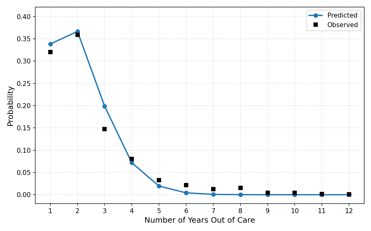
Table 11: Probability of Reengaging
| years | probability | prob_0.8 | prob_0.9 | prob_1.1 | prob_1.2 |
|---|---|---|---|---|---|
| 1 | 0.338 | 0.420 | 0.377 | 0.304 | 0.273 |
| 2 | 0.367 | 0.364 | 0.368 | 0.362 | 0.354 |
| 3 | 0.199 | 0.158 | 0.179 | 0.216 | 0.230 |
| 4 | 0.072 | 0.046 | 0.058 | 0.086 | 0.100 |
| 5 | 0.019 | 0.010 | 0.014 | 0.026 | 0.032 |
| 6 | 0.004 | 0.002 | 0.003 | 0.006 | 0.008 |
| 7 | 0.001 | 0.000 | 0.000 | 0.001 | 0.002 |
| 8 | 0.000 | 0.000 | 0.000 | 0.000 | 0.000 |
| 9 | 0.000 | 0.000 | 0.000 | 0.000 | 0.000 |
| 10 | 0.000 | 0.000 | 0.000 | 0.000 | 0.000 |
| 11 | 0.000 | 0.000 | 0.000 | 0.000 | 0.000 |
| 12 | 0.000 | 0.000 | 0.000 | 0.000 | 0.000 |
When simulated agents are lost to follow up, a number of years out of care is drawn from this distribution and the person will stay lost to follow up until they have spent the correct number of years out of care, they die, or the simulation ends.
CD4 Dynamics In Care </>
A linear regression was used to model the time varying CD4 count of those on ART. To this end, the square root of the time-varying CD4 count (\(\mathrm{sqrt\_cd4n}\)) was modeled as a linear function of age (modeled with a 4-knot restricted cubic spline), CD4 at ART initiation (modeled with a 4-knot restricted cubic spline), number of years since ART initiation (modeled with a 4-knot restricted cubic spline), and interaction terms between CD4 count at ART initiation and number of years since ART initiation.
Age is modeled as a restricted quadratic spline with 4 knots:
\[\mathrm{age}\_1 = \begin{cases} \frac{(\mathrm{age} - k_1)^2 - (\mathrm{age} - k_4)^2}{k_4 - k_1}, & \mathrm{age} \ge k_4\\ \frac{(\mathrm{age} - k_1)^2} {k_4 - k_1}, & k_4 \gt \mathrm{age} \ge k_1\\ 0, & \mathrm{else} \end{cases}\] \[\mathrm{age}\_2 = \begin{cases} \frac{(\mathrm{age} - k_2)^2 - (\mathrm{age} - k_4)^2}{k_4 - k_1}, & \mathrm{age} \ge k_4\\ \frac{(\mathrm{age} - k_2)^2} {k_4 - k_1}, & k_4 \gt \mathrm{age} \ge k_2\\ 0, & \mathrm{else} \end{cases}\] \[\mathrm{age}\_3 = \begin{cases} \frac{(\mathrm{age} - k_3)^2 - (\mathrm{age} - k_4)^2}{k_4 - k_1}, & \mathrm{age} \ge k_4\\ \frac{(\mathrm{age} - k_3)^2} {k_4 - k_1}, & k_4 \gt \mathrm{age} \ge k_3\\ 0, & \mathrm{else} \end{cases}\]CD4 at ART initiation is modeled as a restricted quadratic spline with 4 knots:
\[\mathrm{cd4\_art}\_1 = \begin{cases} \frac{(\mathrm{cd4\_art} - k_1)^2 - (\mathrm{cd4\_art} - k_4)^2}{k_4 - k_1}, & \mathrm{cd4\_art} \ge k_4\\ \frac{(\mathrm{cd4\_art} - k_1)^2} {k_4 - k_1}, & k_4 \gt \mathrm{cd4\_art} \ge k_1\\ 0, & \mathrm{else} \end{cases}\] \[\mathrm{cd4\_art}\_2 = \begin{cases} \frac{(\mathrm{cd4\_art} - k_2)^2 - (\mathrm{cd4\_art} - k_4)^2}{k_4 - k_1}, & \mathrm{cd4\_art} \ge k_4\\ \frac{(\mathrm{cd4\_art} - k_2)^2} {k_4 - k_1}, & k_4 \gt \mathrm{cd4\_art} \ge k_2\\ 0, & \mathrm{else} \end{cases}\] \[\mathrm{cd4\_art}\_3 = \begin{cases} \frac{(\mathrm{cd4\_art} - k_3)^2 - (\mathrm{cd4\_art} - k_4)^2}{k_4 - k_1}, & \mathrm{cd4\_art} \ge k_4\\ \frac{(\mathrm{cd4\_art} - k_3)^2} {k_4 - k_1}, & k_4 \gt \mathrm{cd4\_art} \ge k_3\\ 0, & \mathrm{else} \end{cases}\]The number of years since ART initiation is modeled as a restricted quadratic spline with 4 knots:
\[\mathrm{yrs\_art}\_1 = \begin{cases} \frac{(\mathrm{yrs\_art} - k_1)^2 - (\mathrm{yrs\_art} - k_4)^2}{k_4 - k_1}, & \mathrm{yrs\_art} \ge k_4\\ \frac{(\mathrm{yrs\_art} - k_1)^2} {k_4 - k_1}, & k_4 \gt \mathrm{yrs\_art} \ge k_1\\ 0, & \mathrm{else} \end{cases}\] \[\mathrm{yrs\_art}\_2 = \begin{cases} \frac{(\mathrm{yrs\_art} - k_2)^2 - (\mathrm{yrs\_art} - k_4)^2}{k_4 - k_1}, & \mathrm{yrs\_art} \ge k_4\\ \frac{(\mathrm{yrs\_art} - k_2)^2} {k_4 - k_1}, & k_4 \gt \mathrm{yrs\_art} \ge k_2\\ 0, & \mathrm{else} \end{cases}\] \[\mathrm{yrs\_art}\_3 = \begin{cases} \frac{(\mathrm{yrs\_art} - k_3)^2 - (\mathrm{yrs\_art} - k_4)^2}{k_4 - k_1}, & \mathrm{yrs\_art} \ge k_4\\ \frac{(\mathrm{yrs\_art} - k_3)^2} {k_4 - k_1}, & k_4 \gt \mathrm{yrs\_art} \ge k_3\\ 0, & \mathrm{else} \end{cases}\]The same knot locations were used for each population at $k_1=1$, $k_2=4$, $k_3=7$, and $k_4=13$. The final regression equation resulting from this choice of regressors are as follow:
\[\begin{split} \mathrm{sqrt\_cd4} = \beta_0 &+ \beta_\mathrm{age} \cdot\mathrm{age} + \beta_\mathrm{age\_1} \cdot\mathrm{age\_1} + \beta_\mathrm{age\_2} \cdot\mathrm{age\_2} + \beta_\mathrm{age\_3} \cdot\mathrm{age\_3}\\[2ex] &+ \beta_\mathrm{cd4} \cdot\mathrm{cd4} + \beta_\mathrm{cd4\_1} \cdot\mathrm{cd4\_1} + \beta_\mathrm{cd4\_2} \cdot\mathrm{cd4\_2} + \beta_\mathrm{cd4\_3} \cdot\mathrm{cd4\_3}\\[2ex] &+ \beta_\mathrm{yrs\_art} \cdot\mathrm{yrs\_art} + \beta_\mathrm{yrs\_art\_1} \cdot\mathrm{yrs\_art\_1} + \beta_\mathrm{yrs\_art\_2} \cdot\mathrm{yrs\_art\_2} + \beta_\mathrm{yrs\_art\_3} \cdot\mathrm{yrs\_art\_3}\\[2ex] &+ \beta_\mathrm{cd4\_1\_yrs\_1} \cdot \mathrm{cd4\_1} \cdot \mathrm{yrs\_art\_1} + \beta_\mathrm{cd4\_1\_yrs\_2} \cdot \mathrm{cd4\_1} \cdot \mathrm{yrs\_art\_2}+ \beta_\mathrm{cd4\_1\_yrs\_3} \cdot \mathrm{cd4\_1} \cdot \mathrm{yrs\_art\_3}\\[2ex] &+ \beta_\mathrm{cd4\_2\_yrs\_1} \cdot \mathrm{cd4\_2} \cdot \mathrm{yrs\_art\_1} + \beta_\mathrm{cd4\_2\_yrs\_2} \cdot \mathrm{cd4\_2} \cdot \mathrm{yrs\_art\_2}+ \beta_\mathrm{cd4\_2\_yrs\_3} \cdot \mathrm{cd4\_2} \cdot \mathrm{yrs\_art\_3}\\[2ex] &+ \beta_\mathrm{cd4\_3\_yrs\_1} \cdot \mathrm{cd4\_3} \cdot \mathrm{yrs\_art\_1} + \beta_\mathrm{cd4\_3\_yrs\_2} \cdot \mathrm{cd4\_3} \cdot \mathrm{yrs\_art\_2}+ \beta_\mathrm{cd4\_3\_yrs\_3} \cdot \mathrm{cd4\_3} \cdot \mathrm{yrs\_art\_3} \end{split}\]The coefficients were estimated using a generalized estimating equation (GEE) with an identity link function and an exchangeable correlation structure. The NA-ACCORD population was filtered to those that never left care during study follow-up. Patients who initiated ART before 2000 and who were missing CD4 count data at ART initiation were dropped from analysis. Each remaining patient was assigned a single data point per year for the full range of years 2009 – 2022 and the CD4 count was taken to be the median CD4 count by calendar year. The resulted coefficient estimates are shown in Table 12 and the covariance matrices are shown in Table 16
Table 12: CD4 Increase Coefficient Estimates
| group | (Intercept) | rcs(age, 4)age | rcs(age, 4)age’ | rcs(age, 4)age’’ | rcs(cd4n_ini, 4)cd4n_ini | rcs(cd4n_ini, 4)cd4n_ini’ | rcs(cd4n_ini, 4)cd4n_ini’’ | rcs(cd4n_ini, 4)cd4n_ini’’:rcs(time_from_h1yy, 4)time_from_h1yy | rcs(cd4n_ini, 4)cd4n_ini’‘:rcs(time_from_h1yy, 4)time_from_h1yy’ | rcs(cd4n_ini, 4)cd4n_ini’‘:rcs(time_from_h1yy, 4)time_from_h1yy’’ | rcs(cd4n_ini, 4)cd4n_ini’:rcs(time_from_h1yy, 4)time_from_h1yy | rcs(cd4n_ini, 4)cd4n_ini’:rcs(time_from_h1yy, 4)time_from_h1yy’ | rcs(cd4n_ini, 4)cd4n_ini’:rcs(time_from_h1yy, 4)time_from_h1yy’’ | rcs(cd4n_ini, 4)cd4n_ini:rcs(time_from_h1yy, 4)time_from_h1yy | rcs(cd4n_ini, 4)cd4n_ini:rcs(time_from_h1yy, 4)time_from_h1yy’ | rcs(cd4n_ini, 4)cd4n_ini:rcs(time_from_h1yy, 4)time_from_h1yy’’ | rcs(time_from_h1yy, 4)time_from_h1yy | rcs(time_from_h1yy, 4)time_from_h1yy’ | rcs(time_from_h1yy, 4)time_from_h1yy’’ |
|---|---|---|---|---|---|---|---|---|---|---|---|---|---|---|---|---|---|---|---|
| het_black_female | 10.67 | -0.05 | 0.40 | -1.45 | 0.04 | -0.01 | -0.01 | -0.06 | 0.31 | -0.64 | 0.03 | -0.13 | 0.27 | -0.01 | 0.04 | -0.07 | 2.46 | -7.84 | 14.15 |
| het_black_male | 10.65 | -0.03 | 0.11 | -0.60 | 0.04 | -0.05 | 0.07 | -0.06 | 0.22 | -0.37 | 0.03 | -0.12 | 0.20 | -0.01 | 0.03 | -0.04 | 1.73 | -4.87 | 7.80 |
| het_hisp_female | 15.97 | -0.14 | 0.77 | -2.45 | 0.02 | 0.03 | -0.11 | -0.03 | 0.06 | -0.08 | 0.01 | -0.02 | 0.02 | 0.00 | 0.01 | -0.01 | 1.60 | -3.52 | 5.80 |
| het_hisp_male | 13.71 | -0.08 | 0.14 | -0.41 | 0.03 | 0.04 | -0.08 | -0.07 | 0.35 | -0.74 | 0.04 | -0.22 | 0.45 | -0.01 | 0.03 | -0.06 | 1.60 | -5.00 | 8.70 |
| het_white_female | 12.17 | -0.03 | 0.15 | -0.75 | 0.03 | -0.02 | 0.00 | 0.03 | -0.20 | 0.33 | -0.01 | 0.07 | -0.12 | 0.00 | -0.01 | 0.02 | 1.23 | -2.07 | 3.18 |
| het_white_male | 15.11 | -0.11 | 0.25 | -1.27 | 0.04 | -0.05 | 0.06 | -0.05 | 0.11 | -0.22 | 0.03 | -0.07 | 0.13 | -0.01 | 0.02 | -0.03 | 1.76 | -4.49 | 9.44 |
| idu_black_female | 6.57 | 0.10 | 0.00 | -0.37 | 0.03 | -0.03 | 0.03 | -0.08 | 0.10 | -0.20 | 0.03 | -0.04 | 0.06 | -0.01 | 0.01 | 0.00 | 1.42 | -1.13 | 0.85 |
| idu_black_male | 14.24 | -0.10 | 0.31 | -1.69 | 0.02 | 0.05 | -0.14 | 0.03 | -0.09 | 0.20 | -0.01 | 0.04 | -0.09 | 0.00 | 0.00 | 0.00 | 1.00 | -1.18 | 2.40 |
| idu_hisp_female | 21.21 | -0.28 | 0.35 | -0.87 | 0.03 | 0.00 | -0.07 | 0.14 | -1.37 | 2.45 | -0.05 | 0.48 | -0.86 | 0.01 | -0.09 | 0.17 | 0.29 | 6.40 | -14.28 |
| idu_hisp_male | 13.92 | -0.11 | 0.20 | -0.80 | 0.04 | -0.04 | 0.08 | -0.06 | 0.17 | -0.32 | 0.02 | -0.07 | 0.13 | -0.01 | 0.01 | -0.01 | 1.25 | -0.60 | -0.59 |
| idu_white_female | 13.28 | -0.11 | 0.51 | -2.01 | 0.04 | -0.03 | 0.01 | -0.07 | 0.20 | -0.45 | 0.03 | -0.09 | 0.20 | -0.01 | 0.03 | -0.08 | 1.56 | -4.82 | 12.48 |
| idu_white_male | 13.46 | -0.11 | 0.23 | -1.24 | 0.04 | -0.06 | 0.09 | -0.02 | 0.12 | -0.32 | 0.01 | -0.04 | 0.11 | 0.00 | 0.01 | -0.02 | 1.37 | -2.32 | 4.03 |
| msm_black_male | 12.06 | -0.07 | 0.20 | -0.53 | 0.04 | -0.02 | 0.00 | -0.03 | 0.19 | -0.42 | 0.01 | -0.08 | 0.18 | -0.01 | 0.02 | -0.05 | 1.81 | -6.05 | 11.77 |
| msm_hisp_male | 12.00 | -0.06 | 0.08 | -0.29 | 0.04 | -0.04 | 0.07 | -0.02 | 0.11 | -0.23 | 0.01 | -0.05 | 0.10 | 0.00 | 0.02 | -0.04 | 1.81 | -5.44 | 10.64 |
| msm_white_male | 12.79 | -0.05 | 0.08 | -0.48 | 0.04 | -0.03 | 0.04 | -0.02 | 0.09 | -0.23 | 0.01 | -0.03 | 0.08 | 0.00 | 0.01 | -0.02 | 1.48 | -2.90 | 5.89 |
Table 13: Age Spline Knot Locations
| subgroup | knot_1 | knot_2 | knot_3 | knot_4 |
|---|---|---|---|---|
| het_black_female | 29.00 | 42.00 | 51 | 66 |
| het_black_male | 32.00 | 48.00 | 56 | 69 |
| het_hisp_female | 29.00 | 40.00 | 49 | 65 |
| het_hisp_male | 31.00 | 44.00 | 53 | 68 |
| het_white_female | 29.00 | 44.00 | 53 | 67 |
| het_white_male | 34.00 | 49.00 | 58 | 72 |
| idu_black_female | 38.00 | 50.00 | 57 | 67 |
| idu_black_male | 41.00 | 54.05 | 61 | 69 |
| idu_hisp_female | 34.65 | 48.00 | 56 | 66 |
| idu_hisp_male | 34.00 | 47.00 | 55 | 67 |
| idu_white_female | 33.00 | 45.00 | 52 | 65 |
| idu_white_male | 31.00 | 46.00 | 54 | 66 |
| msm_black_male | 25.00 | 36.00 | 48 | 63 |
| msm_hisp_male | 26.00 | 38.00 | 47 | 62 |
| msm_white_male | 30.00 | 46.00 | 54 | 68 |
Table 14: CD4 Spline Knot Locations
| subgroup | knot_1 | knot_2 | knot_3 | knot_4 |
|---|---|---|---|---|
| het_black_female | 12 | 183.0 | 335 | 719.3 |
| het_black_male | 9 | 136.0 | 303 | 657.0 |
| het_hisp_female | 20 | 207.0 | 359 | 784.0 |
| het_hisp_male | 8 | 89.0 | 239 | 579.0 |
| het_white_female | 22 | 215.0 | 360 | 763.0 |
| het_white_male | 9 | 119.0 | 317 | 671.6 |
| idu_black_female | 8 | 184.0 | 317 | 715.0 |
| idu_black_male | 12 | 154.0 | 329 | 761.0 |
| idu_hisp_female | 24 | 206.1 | 363 | 651.0 |
| idu_hisp_male | 31 | 189.0 | 353 | 653.0 |
| idu_white_female | 29 | 201.0 | 361 | 690.0 |
| idu_white_male | 16 | 177.0 | 329 | 716.0 |
| msm_black_male | 13 | 199.0 | 370 | 765.0 |
| msm_hisp_male | 22 | 207.0 | 373 | 758.4 |
| msm_white_male | 30 | 240.0 | 397 | 790.0 |
Table 15: Age Spline Knot Locations
| subgroup | knot_1 | knot_2 | knot_3 | knot_4 |
|---|---|---|---|---|
| het_black_female | 1 | 4 | 8 | 15 |
| het_black_male | 1 | 4 | 9 | 16 |
| het_hisp_female | 1 | 4 | 8 | 15 |
| het_hisp_male | 1 | 4 | 8 | 16 |
| het_white_female | 1 | 4 | 9 | 16 |
| het_white_male | 1 | 5 | 9 | 17 |
| idu_black_female | 1 | 6 | 10 | 17 |
| idu_black_male | 1 | 6 | 10 | 17 |
| idu_hisp_female | 1 | 3 | 7 | 13 |
| idu_hisp_male | 1 | 5 | 9 | 16 |
| idu_white_female | 1 | 5 | 8 | 15 |
| idu_white_male | 1 | 5 | 9 | 16 |
| msm_black_male | 1 | 4 | 7 | 16 |
| msm_hisp_male | 1 | 4 | 7 | 15 |
| msm_white_male | 1 | 5 | 9 | 16 |
Table 16: CD4 Increase Covariance Matrices
| group | varname | (Intercept) | rcs(age, 4)age | rcs(age, 4)age’ | rcs(age, 4)age’’ | rcs(cd4n_ini, 4)cd4n_ini | rcs(cd4n_ini, 4)cd4n_ini’ | rcs(cd4n_ini, 4)cd4n_ini’’ | rcs(time_from_h1yy, 4)time_from_h1yy | rcs(time_from_h1yy, 4)time_from_h1yy’ | rcs(time_from_h1yy, 4)time_from_h1yy’’ | rcs(cd4n_ini, 4)cd4n_ini:rcs(time_from_h1yy, 4)time_from_h1yy | rcs(cd4n_ini, 4)cd4n_ini’:rcs(time_from_h1yy, 4)time_from_h1yy | rcs(cd4n_ini, 4)cd4n_ini’‘:rcs(time_from_h1yy, 4)time_from_h1yy | rcs(cd4n_ini, 4)cd4n_ini:rcs(time_from_h1yy, 4)time_from_h1yy’ | rcs(cd4n_ini, 4)cd4n_ini’:rcs(time_from_h1yy, 4)time_from_h1yy’ | rcs(cd4n_ini, 4)cd4n_ini’‘:rcs(time_from_h1yy, 4)time_from_h1yy’ | rcs(cd4n_ini, 4)cd4n_ini:rcs(time_from_h1yy, 4)time_from_h1yy’’ | rcs(cd4n_ini, 4)cd4n_ini’:rcs(time_from_h1yy, 4)time_from_h1yy’’ | rcs(cd4n_ini, 4)cd4n_ini’‘:rcs(time_from_h1yy, 4)time_from_h1yy’’ |
|---|---|---|---|---|---|---|---|---|---|---|---|---|---|---|---|---|---|---|---|---|
| het_black_female | (Intercept) | 0.945246509 | -0.021234239 | 0.057339439 | -0.178161473 | -0.001592247 | 0.005511022 | -0.012257957 | -0.04481439 | 0.146252756 | -0.272918774 | 0.000351007 | -0.001231117 | 0.002735874 | -0.00113566 | 0.004076262 | -0.009138423 | 0.002112031 | -0.007643653 | 0.017212017 |
| het_black_female | rcs(age, 4)age | -0.021234239 | 0.000599454 | -0.001728817 | 0.005497105 | 5.92E-06 | -8.13E-06 | 9.84E-06 | -6.80E-06 | 0.00089194 | -0.001756471 | -1.22E-07 | -2.54E-06 | 8.04E-06 | -6.21E-06 | 3.11E-05 | -7.66E-05 | 1.25E-05 | -6.02E-05 | 0.000145779 |
| het_black_female | rcs(age, 4)age’ | 0.057339439 | -0.001728817 | 0.006246235 | -0.021475055 | -1.31E-05 | 2.14E-05 | -3.31E-05 | -0.00010192 | -0.002895695 | 0.005826867 | -3.56E-07 | 1.05E-05 | -3.08E-05 | 2.48E-05 | -0.00012416 | 0.000306428 | -5.06E-05 | 0.00024595 | -0.000599393 |
| het_black_female | rcs(age, 4)age’’ | -0.178161473 | 0.005497105 | -0.021475055 | 0.077170859 | 3.31E-05 | -4.66E-05 | 6.34E-05 | 0.000215588 | 0.00884281 | -0.017840626 | 2.24E-06 | -3.70E-05 | 0.000106534 | -8.32E-05 | 0.000425333 | -0.001056503 | 0.000168387 | -0.000841515 | 0.002066785 |
| het_black_female | rcs(cd4n_ini, 4)cd4n_ini | -0.001592247 | 5.92E-06 | -1.31E-05 | 3.31E-05 | 1.34E-05 | -5.78E-05 | 0.000136495 | 0.000344337 | -0.001326612 | 0.002498236 | -3.33E-06 | 1.44E-05 | -3.39E-05 | 1.29E-05 | -5.60E-05 | 0.00013223 | -2.44E-05 | 0.000105875 | -0.000249973 |
| het_black_female | rcs(cd4n_ini, 4)cd4n_ini’ | 0.005511022 | -8.13E-06 | 2.14E-05 | -4.66E-05 | -5.78E-05 | 0.000271593 | -0.000655298 | -0.001308663 | 0.005050464 | -0.009517634 | 1.44E-05 | -6.69E-05 | 0.000160829 | -5.60E-05 | 0.000261255 | -0.000628544 | 0.000105849 | -0.000493977 | 0.00118887 |
| het_black_female | rcs(cd4n_ini, 4)cd4n_ini’’ | -0.012257957 | 9.84E-06 | -3.31E-05 | 6.34E-05 | 0.000136495 | -0.000655298 | 0.00159152 | 0.002989357 | -0.011538104 | 0.021747503 | -3.38E-05 | 0.000160797 | -0.000389134 | 0.00013217 | -0.000628208 | 0.001519932 | -0.000249727 | 0.001187893 | -0.002875001 |
| het_black_female | rcs(time_from_h1yy, 4)time_from_h1yy | -0.04481439 | -6.80E-06 | -0.00010192 | 0.000215588 | 0.000344337 | -0.001308663 | 0.002989357 | 0.026825428 | -0.132383834 | 0.258675987 | -0.000202664 | 0.000771517 | -0.001763223 | 0.001001723 | -0.003821538 | 0.008742103 | -0.001957753 | 0.007474226 | -0.017103996 |
| het_black_female | rcs(time_from_h1yy, 4)time_from_h1yy’ | 0.146252756 | 0.00089194 | -0.002895695 | 0.00884281 | -0.001326612 | 0.005050464 | -0.011538104 | -0.132383834 | 0.862644548 | -1.777086869 | 0.001002014 | -0.00382255 | 0.00874374 | -0.006546039 | 0.025106534 | -0.057545186 | 0.01350365 | -0.051869229 | 0.118951018 |
| het_black_female | rcs(time_from_h1yy, 4)time_from_h1yy’’ | -0.272918774 | -0.001756471 | 0.005826867 | -0.017840626 | 0.002498236 | -0.009517634 | 0.021747503 | 0.258675987 | -1.777086869 | 3.706869575 | -0.00195807 | 0.007472713 | -0.017096636 | 0.013497456 | -0.051832405 | 0.118856615 | -0.02820944 | 0.108547777 | -0.249084635 |
| het_black_female | rcs(cd4n_ini, 4)cd4n_ini:rcs(time_from_h1yy, 4)time_from_h1yy | 0.000351007 | -1.22E-07 | -3.56E-07 | 2.24E-06 | -3.33E-06 | 1.44E-05 | -3.38E-05 | -0.000202664 | 0.001002014 | -0.00195807 | 1.96E-06 | -8.50E-06 | 2.01E-05 | -9.63E-06 | 4.17E-05 | -9.84E-05 | 1.88E-05 | -8.12E-05 | 0.000191735 |
| het_black_female | rcs(cd4n_ini, 4)cd4n_ini’:rcs(time_from_h1yy, 4)time_from_h1yy | -0.001231117 | -2.54E-06 | 1.05E-05 | -3.70E-05 | 1.44E-05 | -6.69E-05 | 0.000160797 | 0.000771517 | -0.00382255 | 0.007472713 | -8.50E-06 | 3.98E-05 | -9.57E-05 | 4.17E-05 | -0.000194844 | 0.00046952 | -8.12E-05 | 0.000379575 | -0.000914903 |
| het_black_female | rcs(cd4n_ini, 4)cd4n_ini’‘:rcs(time_from_h1yy, 4)time_from_h1yy | 0.002735874 | 8.04E-06 | -3.08E-05 | 0.000106534 | -3.39E-05 | 0.000160829 | -0.000389134 | -0.001763223 | 0.00874374 | -0.017096636 | 2.01E-05 | -9.57E-05 | 0.000231901 | -9.84E-05 | 0.000469454 | -0.001138379 | 0.000191646 | -0.000914744 | 0.002219006 |
| het_black_female | rcs(cd4n_ini, 4)cd4n_ini:rcs(time_from_h1yy, 4)time_from_h1yy’ | -0.00113566 | -6.21E-06 | 2.48E-05 | -8.32E-05 | 1.29E-05 | -5.60E-05 | 0.00013217 | 0.001001723 | -0.006546039 | 0.013497456 | -9.63E-06 | 4.17E-05 | -9.84E-05 | 6.24E-05 | -0.000270548 | 0.000639545 | -0.000128538 | 0.000557751 | -0.001318905 |
| het_black_female | rcs(cd4n_ini, 4)cd4n_ini’:rcs(time_from_h1yy, 4)time_from_h1yy’ | 0.004076262 | 3.11E-05 | -0.00012416 | 0.000425333 | -5.60E-05 | 0.000261255 | -0.000628208 | -0.003821538 | 0.025106534 | -0.051832405 | 4.17E-05 | -0.000194844 | 0.000469454 | -0.000270548 | 0.001271677 | -0.003071227 | 0.000557754 | -0.002625605 | 0.006345264 |
| het_black_female | rcs(cd4n_ini, 4)cd4n_ini’‘:rcs(time_from_h1yy, 4)time_from_h1yy’ | -0.009138423 | -7.66E-05 | 0.000306428 | -0.001056503 | 0.00013223 | -0.000628544 | 0.001519932 | 0.008742103 | -0.057545186 | 0.118856615 | -9.84E-05 | 0.00046952 | -0.001138379 | 0.000639545 | -0.003071227 | 0.007468855 | -0.001318928 | 0.00634533 | -0.015443936 |
| het_black_female | rcs(cd4n_ini, 4)cd4n_ini:rcs(time_from_h1yy, 4)time_from_h1yy’’ | 0.002112031 | 1.25E-05 | -5.06E-05 | 0.000168387 | -2.44E-05 | 0.000105849 | -0.000249727 | -0.001957753 | 0.01350365 | -0.02820944 | 1.88E-05 | -8.12E-05 | 0.000191646 | -0.000128538 | 0.000557754 | -0.001318928 | 0.000268738 | -0.001168115 | 0.002763949 |
| het_black_female | rcs(cd4n_ini, 4)cd4n_ini’:rcs(time_from_h1yy, 4)time_from_h1yy’’ | -0.007643653 | -6.02E-05 | 0.00024595 | -0.000841515 | 0.000105875 | -0.000493977 | 0.001187893 | 0.007474226 | -0.051869229 | 0.108547777 | -8.12E-05 | 0.000379575 | -0.000914744 | 0.000557751 | -0.002625605 | 0.00634533 | -0.001168115 | 0.005515092 | -0.013341831 |
| het_black_female | rcs(cd4n_ini, 4)cd4n_ini’‘:rcs(time_from_h1yy, 4)time_from_h1yy’’ | 0.017212017 | 0.000145779 | -0.000599393 | 0.002066785 | -0.000249973 | 0.00118887 | -0.002875001 | -0.017103996 | 0.118951018 | -0.249084635 | 0.000191735 | -0.000914903 | 0.002219006 | -0.001318905 | 0.006345264 | -0.015443936 | 0.002763949 | -0.013341831 | 0.032512122 |
| het_black_male | (Intercept) | 0.930349892 | -0.019187795 | 0.041202289 | -0.174061707 | -0.001840601 | 0.008143175 | -0.014975348 | -0.043395794 | 0.150386876 | -0.251289692 | 0.000433578 | -0.002022006 | 0.00375066 | -0.001600853 | 0.008079541 | -0.015246795 | 0.002681522 | -0.013846384 | 0.026254056 |
| het_black_male | rcs(age, 4)age | -0.019187795 | 0.000488209 | -0.001108958 | 0.004789707 | 6.35E-06 | -1.27E-05 | 1.76E-05 | 1.55E-05 | 0.000797777 | -0.001633349 | -5.01E-07 | 4.85E-07 | -3.54E-08 | -3.70E-06 | 1.03E-05 | -1.68E-05 | 8.90E-06 | -2.22E-05 | 3.42E-05 |
| het_black_male | rcs(age, 4)age’ | 0.041202289 | -0.001108958 | 0.003291914 | -0.015769404 | -1.48E-05 | 2.94E-05 | -4.15E-05 | -0.000261866 | -0.001674972 | 0.003662925 | 1.18E-06 | 1.31E-07 | -2.67E-06 | 7.11E-06 | -1.45E-05 | 1.99E-05 | -1.85E-05 | 3.37E-05 | -4.11E-05 |
| het_black_male | rcs(age, 4)age’’ | -0.174061707 | 0.004789707 | -0.015769404 | 0.081740396 | 6.09E-05 | -0.000109077 | 0.000144856 | 0.001355359 | 0.006525474 | -0.015235628 | -6.13E-06 | -9.51E-07 | 1.30E-05 | -2.58E-05 | 3.63E-05 | -2.35E-05 | 7.22E-05 | -0.000102701 | 7.19E-05 |
| het_black_male | rcs(cd4n_ini, 4)cd4n_ini | -0.001840601 | 6.35E-06 | -1.48E-05 | 6.09E-05 | 2.04E-05 | -0.000112394 | 0.000215625 | 0.000414553 | -0.001739016 | 0.003014395 | -5.07E-06 | 2.75E-05 | -5.26E-05 | 2.15E-05 | -0.000117463 | 0.000225443 | -3.74E-05 | 0.000204869 | -0.000393468 |
| het_black_male | rcs(cd4n_ini, 4)cd4n_ini’ | 0.008143175 | -1.27E-05 | 2.94E-05 | -0.000109077 | -0.000112394 | 0.000668326 | -0.001302921 | -0.001998223 | 0.008468994 | -0.014701927 | 2.75E-05 | -0.000159966 | 0.000310819 | -0.000117232 | 0.000687815 | -0.001340823 | 0.000204487 | -0.001203433 | 0.002348128 |
| het_black_male | rcs(cd4n_ini, 4)cd4n_ini’’ | -0.014975348 | 1.76E-05 | -4.15E-05 | 0.000144856 | 0.000215625 | -0.001302921 | 0.002549788 | 0.003736784 | -0.015876648 | 0.027572451 | -5.26E-05 | 0.000310695 | -0.000605896 | 0.000224797 | -0.001339535 | 0.002621754 | -0.000392366 | 0.002345768 | -0.004595812 |
| het_black_male | rcs(time_from_h1yy, 4)time_from_h1yy | -0.043395794 | 1.55E-05 | -0.000261866 | 0.001355359 | 0.000414553 | -0.001998223 | 0.003736784 | 0.021369439 | -0.102880603 | 0.181250929 | -0.000203543 | 0.000988365 | -0.001852511 | 0.00098825 | -0.004824213 | 0.009058817 | -0.001742721 | 0.008514914 | -0.015993834 |
| het_black_male | rcs(time_from_h1yy, 4)time_from_h1yy’ | 0.150386876 | 0.000797777 | -0.001674972 | 0.006525473 | -0.001739016 | 0.008468994 | -0.015876648 | -0.102880603 | 0.609947322 | -1.121379198 | 0.000987308 | -0.004817983 | 0.009044785 | -0.005860119 | 0.028695699 | -0.053946394 | 0.01077489 | -0.052772314 | 0.099217419 |
| het_black_male | rcs(time_from_h1yy, 4)time_from_h1yy’’ | -0.251289692 | -0.001633349 | 0.003662925 | -0.015235628 | 0.003014395 | -0.014701927 | 0.027572451 | 0.181250929 | -1.121379198 | 2.087553788 | -0.001740809 | 0.008502666 | -0.015966124 | 0.010772094 | -0.052764966 | 0.099202734 | -0.020050028 | 0.09820981 | -0.184643364 |
| het_black_male | rcs(cd4n_ini, 4)cd4n_ini:rcs(time_from_h1yy, 4)time_from_h1yy | 0.000433578 | -5.01E-07 | 1.18E-06 | -6.13E-06 | -5.07E-06 | 2.75E-05 | -5.26E-05 | -0.000203543 | 0.000987308 | -0.001740809 | 2.56E-06 | -1.41E-05 | 2.72E-05 | -1.26E-05 | 6.98E-05 | -0.000134619 | 2.22E-05 | -0.000123716 | 0.00023855 |
| het_black_male | rcs(cd4n_ini, 4)cd4n_ini’:rcs(time_from_h1yy, 4)time_from_h1yy | -0.002022006 | 4.85E-07 | 1.31E-07 | -9.51E-07 | 2.75E-05 | -0.000159966 | 0.000310695 | 0.000988365 | -0.004817983 | 0.008502666 | -1.41E-05 | 8.41E-05 | -0.000164233 | 6.98E-05 | -0.000419043 | 0.000821197 | -0.000123632 | 0.000743893 | -0.001458699 |
| het_black_male | rcs(cd4n_ini, 4)cd4n_ini’‘:rcs(time_from_h1yy, 4)time_from_h1yy | 0.00375066 | -3.54E-08 | -2.67E-06 | 1.30E-05 | -5.26E-05 | 0.000310819 | -0.000605896 | -0.001852511 | 0.009044785 | -0.015966124 | 2.72E-05 | -0.000164233 | 0.000322013 | -0.000134462 | 0.00082078 | -0.001615453 | 0.000238275 | -0.001457931 | 0.002871397 |
| het_black_male | rcs(cd4n_ini, 4)cd4n_ini:rcs(time_from_h1yy, 4)time_from_h1yy’ | -0.001600853 | -3.70E-06 | 7.11E-06 | -2.58E-05 | 2.15E-05 | -0.000117232 | 0.000224797 | 0.00098825 | -0.005860119 | 0.010772094 | -1.26E-05 | 6.98E-05 | -0.000134462 | 7.68E-05 | -0.000433491 | 0.000838349 | -0.000142037 | 0.000804533 | -0.001556753 |
| het_black_male | rcs(cd4n_ini, 4)cd4n_ini’:rcs(time_from_h1yy, 4)time_from_h1yy’ | 0.008079541 | 1.03E-05 | -1.45E-05 | 3.63E-05 | -0.000117463 | 0.000687815 | -0.001339535 | -0.004824213 | 0.028695699 | -0.052764966 | 6.98E-05 | -0.000419043 | 0.00082078 | -0.000433491 | 0.002660851 | -0.005239906 | 0.000804548 | -0.004959001 | 0.009772736 |
| het_black_male | rcs(cd4n_ini, 4)cd4n_ini’‘:rcs(time_from_h1yy, 4)time_from_h1yy’ | -0.015246795 | -1.68E-05 | 1.99E-05 | -2.35E-05 | 0.000225443 | -0.001340823 | 0.002621754 | 0.009058817 | -0.053946394 | 0.099202734 | -0.000134619 | 0.000821197 | -0.001615453 | 0.000838349 | -0.005239906 | 0.010368196 | -0.00155678 | 0.009772788 | -0.019352489 |
| het_black_male | rcs(cd4n_ini, 4)cd4n_ini:rcs(time_from_h1yy, 4)time_from_h1yy’’ | 0.002681522 | 8.90E-06 | -1.85E-05 | 7.22E-05 | -3.74E-05 | 0.000204487 | -0.000392366 | -0.001742721 | 0.01077489 | -0.020050028 | 2.22E-05 | -0.000123632 | 0.000238275 | -0.000142037 | 0.000804548 | -0.00155678 | 0.000266323 | -0.001513074 | 0.002929159 |
| het_black_male | rcs(cd4n_ini, 4)cd4n_ini’:rcs(time_from_h1yy, 4)time_from_h1yy’’ | -0.013846384 | -2.22E-05 | 3.37E-05 | -0.000102701 | 0.000204869 | -0.001203433 | 0.002345768 | 0.008514914 | -0.052772314 | 0.09820981 | -0.000123716 | 0.000743893 | -0.001457931 | 0.000804533 | -0.004959001 | 0.009772788 | -0.001513074 | 0.009367442 | -0.018472949 |
| het_black_male | rcs(cd4n_ini, 4)cd4n_ini’‘:rcs(time_from_h1yy, 4)time_from_h1yy’’ | 0.026254056 | 3.42E-05 | -4.11E-05 | 7.19E-05 | -0.000393468 | 0.002348128 | -0.004595812 | -0.015993834 | 0.099217419 | -0.184643364 | 0.00023855 | -0.001458699 | 0.002871397 | -0.001556753 | 0.009772736 | -0.019352489 | 0.002929159 | -0.018472949 | 0.036606857 |
| het_hisp_female | (Intercept) | 4.601714247 | -0.100546917 | 0.330178438 | -0.89568551 | -0.00820612 | 0.028352683 | -0.065664477 | -0.346888677 | 1.425756849 | -2.685194864 | 0.002185509 | -0.007236891 | 0.016496576 | -0.008018604 | 0.023883815 | -0.052034961 | 0.014564567 | -0.040996691 | 0.086829796 |
| het_hisp_female | rcs(age, 4)age | -0.100546917 | 0.00292686 | -0.01032742 | 0.028640477 | 2.74E-05 | -1.48E-05 | -3.32E-05 | 0.002728946 | -0.015682363 | 0.030688032 | -1.47E-05 | 2.02E-05 | -2.05E-05 | 6.16E-05 | -1.69E-05 | -0.000128222 | -0.000107386 | -5.85E-05 | 0.000505942 |
| het_hisp_female | rcs(age, 4)age’ | 0.330178438 | -0.01032742 | 0.046118061 | -0.136787313 | -8.49E-05 | 0.000114533 | -0.000116205 | -0.009544086 | 0.052850145 | -0.102180274 | 5.00E-05 | -4.29E-05 | -1.25E-05 | -0.000222854 | -3.57E-05 | 0.000766647 | 0.000382397 | 0.000405753 | -0.002419933 |
| het_hisp_female | rcs(age, 4)age’’ | -0.89568551 | 0.028640477 | -0.136787313 | 0.418009057 | 0.000217441 | -0.000349536 | 0.000470044 | 0.02343291 | -0.13902898 | 0.266061831 | -0.000129404 | 7.62E-05 | 0.000152114 | 0.00062308 | 0.00011026 | -0.0021981 | -0.001058075 | -0.001153275 | 0.00682513 |
| het_hisp_female | rcs(cd4n_ini, 4)cd4n_ini | -0.00820612 | 2.74E-05 | -8.49E-05 | 0.000217441 | 5.99E-05 | -0.000262613 | 0.00065355 | 0.001706384 | -0.006050258 | 0.011144904 | -1.38E-05 | 6.09E-05 | -0.000152019 | 5.03E-05 | -0.000223214 | 0.000557773 | -9.30E-05 | 0.00041302 | -0.001031917 |
| het_hisp_female | rcs(cd4n_ini, 4)cd4n_ini’ | 0.028352683 | -1.48E-05 | 0.000114533 | -0.000349536 | -0.000262613 | 0.001290441 | -0.003313573 | -0.006511383 | 0.023087825 | -0.042491772 | 6.08E-05 | -0.000304025 | 0.000786012 | -0.000223604 | 0.001128449 | -0.002922212 | 0.000414336 | -0.002093773 | 0.005422701 |
| het_hisp_female | rcs(cd4n_ini, 4)cd4n_ini’’ | -0.065664477 | -3.32E-05 | -0.000116205 | 0.000470044 | 0.00065355 | -0.003313573 | 0.008586116 | 0.015622691 | -0.055363613 | 0.101854783 | -0.000151817 | 0.000785838 | -0.002052618 | 0.000559153 | -0.002923302 | 0.007649228 | -0.001036407 | 0.005426413 | -0.014201909 |
| het_hisp_female | rcs(time_from_h1yy, 4)time_from_h1yy | -0.346888677 | 0.002728946 | -0.009544086 | 0.02343291 | 0.001706384 | -0.006511383 | 0.015622691 | 0.133016303 | -0.584451241 | 1.128644681 | -0.000879571 | 0.003388603 | -0.008148841 | 0.003911502 | -0.015215596 | 0.036676705 | -0.007561834 | 0.029445729 | -0.070990722 |
| het_hisp_female | rcs(time_from_h1yy, 4)time_from_h1yy’ | 1.425756849 | -0.015682363 | 0.052850145 | -0.13902898 | -0.006050258 | 0.023087825 | -0.055363613 | -0.584451241 | 3.344107427 | -6.875270416 | 0.003922817 | -0.015242571 | 0.036729318 | -0.022672334 | 0.089379726 | -0.216307017 | 0.046623849 | -0.18402324 | 0.445525561 |
| het_hisp_female | rcs(time_from_h1yy, 4)time_from_h1yy’’ | -2.685194864 | 0.030688032 | -0.102180274 | 0.266061831 | 0.011144904 | -0.042491772 | 0.101854783 | 1.128644681 | -6.875270416 | 14.40605336 | -0.00758633 | 0.029508255 | -0.071124376 | 0.046634955 | -0.1840257 | 0.445516811 | -0.097690608 | 0.385854449 | -0.934451507 |
| het_hisp_female | rcs(cd4n_ini, 4)cd4n_ini:rcs(time_from_h1yy, 4)time_from_h1yy | 0.002185509 | -1.47E-05 | 5.00E-05 | -0.000129404 | -1.38E-05 | 6.08E-05 | -0.000151817 | -0.000879571 | 0.003922817 | -0.00758633 | 7.34E-06 | -3.28E-05 | 8.21E-05 | -3.33E-05 | 0.000150199 | -0.000376347 | 6.45E-05 | -0.000291045 | 0.000729257 |
| het_hisp_female | rcs(cd4n_ini, 4)cd4n_ini’:rcs(time_from_h1yy, 4)time_from_h1yy | -0.007236891 | 2.02E-05 | -4.29E-05 | 7.62E-05 | 6.09E-05 | -0.000304025 | 0.000785838 | 0.003388603 | -0.015242571 | 0.029508255 | -3.28E-05 | 0.000165507 | -0.000428 | 0.000150315 | -0.000762822 | 0.001973486 | -0.000291382 | 0.001478277 | -0.003823747 |
| het_hisp_female | rcs(cd4n_ini, 4)cd4n_ini’‘:rcs(time_from_h1yy, 4)time_from_h1yy | 0.016496576 | -2.05E-05 | -1.25E-05 | 0.000152114 | -0.000152019 | 0.000786012 | -0.002052618 | -0.008148841 | 0.036729318 | -0.071124376 | 8.21E-05 | -0.000428 | 0.001117653 | -0.000376742 | 0.001973921 | -0.005156708 | 0.000730402 | -0.003824896 | 0.009990513 |
| het_hisp_female | rcs(cd4n_ini, 4)cd4n_ini:rcs(time_from_h1yy, 4)time_from_h1yy’ | -0.008018604 | 6.16E-05 | -0.000222854 | 0.00062308 | 5.03E-05 | -0.000223604 | 0.000559153 | 0.003911502 | -0.022672334 | 0.046634955 | -3.33E-05 | 0.000150315 | -0.000376742 | 0.000196924 | -0.000901361 | 0.002267341 | -0.000404886 | 0.001854234 | -0.004665158 |
| het_hisp_female | rcs(cd4n_ini, 4)cd4n_ini’:rcs(time_from_h1yy, 4)time_from_h1yy’ | 0.023883815 | -1.69E-05 | -3.57E-05 | 0.00011026 | -0.000223214 | 0.001128449 | -0.002923302 | -0.015215596 | 0.089379726 | -0.1840257 | 0.000150199 | -0.000762822 | 0.001973921 | -0.000901361 | 0.004631569 | -0.012013866 | 0.001854411 | -0.009525534 | 0.024707727 |
| het_hisp_female | rcs(cd4n_ini, 4)cd4n_ini’‘:rcs(time_from_h1yy, 4)time_from_h1yy’ | -0.052034961 | -0.000128222 | 0.000766647 | -0.0021981 | 0.000557773 | -0.002922212 | 0.007649228 | 0.036676705 | -0.216307017 | 0.445516811 | -0.000376347 | 0.001973486 | -0.005156708 | 0.002267341 | -0.012013866 | 0.031467749 | -0.004665745 | 0.024707905 | -0.064715095 |
| het_hisp_female | rcs(cd4n_ini, 4)cd4n_ini:rcs(time_from_h1yy, 4)time_from_h1yy’’ | 0.014564567 | -0.000107386 | 0.000382397 | -0.001058075 | -9.30E-05 | 0.000414336 | -0.001036407 | -0.007561834 | 0.046623849 | -0.097690608 | 6.45E-05 | -0.000291382 | 0.000730402 | -0.000404886 | 0.001854411 | -0.004665745 | 0.000846988 | -0.003879585 | 0.009762359 |
| het_hisp_female | rcs(cd4n_ini, 4)cd4n_ini’:rcs(time_from_h1yy, 4)time_from_h1yy’’ | -0.040996691 | -5.85E-05 | 0.000405753 | -0.001153275 | 0.00041302 | -0.002093773 | 0.005426413 | 0.029445729 | -0.18402324 | 0.385854449 | -0.000291045 | 0.001478277 | -0.003824896 | 0.001854234 | -0.009525534 | 0.024707905 | -0.003879585 | 0.01991397 | -0.051649574 |
| het_hisp_female | rcs(cd4n_ini, 4)cd4n_ini’‘:rcs(time_from_h1yy, 4)time_from_h1yy’’ | 0.086829796 | 0.000505942 | -0.002419933 | 0.00682513 | -0.001031917 | 0.005422701 | -0.014201909 | -0.070990722 | 0.445525561 | -0.934451507 | 0.000729257 | -0.003823747 | 0.009990513 | -0.004665158 | 0.024707727 | -0.064715095 | 0.009762359 | -0.051649574 | 0.135268812 |
| het_hisp_male | (Intercept) | 2.709933555 | -0.064740678 | 0.184444489 | -0.582021792 | -0.005869062 | 0.045722216 | -0.074362994 | -0.084335019 | 0.506400315 | -1.047521951 | 0.001407894 | -0.01235579 | 0.020593568 | -0.006117877 | 0.048072329 | -0.079303557 | 0.011335895 | -0.082826701 | 0.13545393 |
| het_hisp_male | rcs(age, 4)age | -0.064740678 | 0.001864469 | -0.005536102 | 0.017786914 | 6.66E-06 | -0.000133708 | 0.000246176 | -0.000484356 | -0.002225921 | 0.007332712 | -3.10E-06 | 7.92E-05 | -0.000148072 | 1.26E-05 | -0.000148145 | 0.000288214 | -2.17E-05 | 6.95E-05 | -0.000160661 |
| het_hisp_male | rcs(age, 4)age’ | 0.184444489 | -0.005536102 | 0.020355975 | -0.070648151 | -5.89E-05 | 0.000726976 | -0.001260045 | 0.001275819 | 0.00512579 | -0.019220023 | 1.11E-05 | -0.000265378 | 0.00049135 | -1.81E-05 | 0.000225199 | -0.000493365 | 2.62E-05 | 0.000321059 | -0.00042876 |
| het_hisp_male | rcs(age, 4)age’’ | -0.582021792 | 0.017786914 | -0.070648151 | 0.256409525 | 0.000219738 | -0.002688694 | 0.004618256 | -0.004644135 | -0.010531615 | 0.048529588 | -3.37E-05 | 0.000804796 | -0.001492052 | -3.88E-05 | 0.000453543 | -0.00042552 | 0.000120956 | -0.003641066 | 0.005845896 |
| het_hisp_male | rcs(cd4n_ini, 4)cd4n_ini | -0.005869062 | 6.66E-06 | -5.89E-05 | 0.000219738 | 0.000102123 | -0.000849637 | 0.001387216 | 0.001309735 | -0.005648788 | 0.010534493 | -2.32E-05 | 0.000197024 | -0.000323594 | 0.000101746 | -0.000869904 | 0.001430284 | -0.000189994 | 0.001624334 | -0.002669947 |
| het_hisp_male | rcs(cd4n_ini, 4)cd4n_ini’ | 0.045722216 | -0.000133708 | 0.000726976 | -0.002688694 | -0.000849637 | 0.007585185 | -0.012528714 | -0.009642363 | 0.042283687 | -0.079120957 | 0.000195968 | -0.001795077 | 0.002987728 | -0.000864487 | 0.00796725 | -0.013270683 | 0.001614844 | -0.014867865 | 0.024752179 |
| het_hisp_male | rcs(cd4n_ini, 4)cd4n_ini’’ | -0.074362994 | 0.000246176 | -0.001260045 | 0.004618256 | 0.001387216 | -0.012528714 | 0.020739436 | 0.015488389 | -0.068104908 | 0.127496353 | -0.000321339 | 0.002982848 | -0.004977878 | 0.001419253 | -0.013252249 | 0.022131736 | -0.002650949 | 0.024724119 | -0.041267448 |
| het_hisp_male | rcs(time_from_h1yy, 4)time_from_h1yy | -0.084335019 | -0.000484356 | 0.001275819 | -0.004644135 | 0.001309735 | -0.009642363 | 0.015488389 | 0.050385883 | -0.247450526 | 0.46474967 | -0.000636971 | 0.004702467 | -0.007564195 | 0.003157422 | -0.023326102 | 0.037496594 | -0.00594719 | 0.043968588 | -0.070672302 |
| het_hisp_male | rcs(time_from_h1yy, 4)time_from_h1yy’ | 0.506400315 | -0.002225921 | 0.00512579 | -0.010531615 | -0.005648788 | 0.042283687 | -0.068104908 | -0.247450526 | 1.596948931 | -3.189713897 | 0.003154196 | -0.023297083 | 0.037462762 | -0.01999203 | 0.145475221 | -0.233059946 | 0.039771725 | -0.288526828 | 0.461882748 |
| het_hisp_male | rcs(time_from_h1yy, 4)time_from_h1yy’’ | -1.047521951 | 0.007332712 | -0.019220023 | 0.048529588 | 0.010534493 | -0.079120957 | 0.127496353 | 0.46474967 | -3.189713897 | 6.481747118 | -0.005939778 | 0.043920885 | -0.07063348 | 0.039789876 | -0.288805365 | 0.46241495 | -0.080422489 | 0.581522742 | -0.930246619 |
| het_hisp_male | rcs(cd4n_ini, 4)cd4n_ini:rcs(time_from_h1yy, 4)time_from_h1yy | 0.001407894 | -3.10E-06 | 1.11E-05 | -3.37E-05 | -2.32E-05 | 0.000195968 | -0.000321339 | -0.000636971 | 0.003154196 | -0.005939778 | 1.14E-05 | -9.75E-05 | 0.00016039 | -5.81E-05 | 0.000498621 | -0.000819523 | 0.000110331 | -0.000948569 | 0.001558698 |
| het_hisp_male | rcs(cd4n_ini, 4)cd4n_ini’:rcs(time_from_h1yy, 4)time_from_h1yy | -0.01235579 | 7.92E-05 | -0.000265378 | 0.000804796 | 0.000197024 | -0.001795077 | 0.002982848 | 0.004702467 | -0.023297083 | 0.043920885 | -9.75E-05 | 0.000910391 | -0.001520052 | 0.000499073 | -0.004668046 | 0.007780941 | -0.000949803 | 0.008889389 | -0.014810903 |
| het_hisp_male | rcs(cd4n_ini, 4)cd4n_ini’‘:rcs(time_from_h1yy, 4)time_from_h1yy | 0.020593568 | -0.000148072 | 0.00049135 | -0.001492052 | -0.000323594 | 0.002987728 | -0.004977878 | -0.007564195 | 0.037462762 | -0.07063348 | 0.00016039 | -0.001520052 | 0.002545327 | -0.000820617 | 0.007784876 | -0.01301126 | 0.001561631 | -0.014820916 | 0.024758915 |
| het_hisp_male | rcs(cd4n_ini, 4)cd4n_ini:rcs(time_from_h1yy, 4)time_from_h1yy’ | -0.006117877 | 1.26E-05 | -1.81E-05 | -3.88E-05 | 0.000101746 | -0.000864487 | 0.001419253 | 0.003157422 | -0.01999203 | 0.039789876 | -5.81E-05 | 0.000499073 | -0.000820617 | 0.000376774 | -0.00322755 | 0.005291568 | -0.000753367 | 0.006449205 | -0.010567177 |
| het_hisp_male | rcs(cd4n_ini, 4)cd4n_ini’:rcs(time_from_h1yy, 4)time_from_h1yy’ | 0.048072329 | -0.000148145 | 0.000225199 | 0.000453543 | -0.000869904 | 0.00796725 | -0.013252249 | -0.023326102 | 0.145475222 | -0.288805365 | 0.000498621 | -0.004668046 | 0.007784876 | -0.00322755 | 0.030086634 | -0.049981329 | 0.006451639 | -0.060103228 | 0.099769136 |
| het_hisp_male | rcs(cd4n_ini, 4)cd4n_ini’‘:rcs(time_from_h1yy, 4)time_from_h1yy’ | -0.079303557 | 0.000288214 | -0.000493365 | -0.00042552 | 0.001430284 | -0.013270683 | 0.022131736 | 0.037496594 | -0.233059946 | 0.46241495 | -0.000819523 | 0.007780941 | -0.01301126 | 0.005291568 | -0.049981329 | 0.083230377 | -0.010572572 | 0.099783406 | -0.166023099 |
| het_hisp_male | rcs(cd4n_ini, 4)cd4n_ini:rcs(time_from_h1yy, 4)time_from_h1yy’’ | 0.011335895 | -2.17E-05 | 2.62E-05 | 0.000120956 | -0.000189994 | 0.001614844 | -0.002650949 | -0.00594719 | 0.039771725 | -0.080422489 | 0.000110331 | -0.000949803 | 0.001561631 | -0.000753367 | 0.006451639 | -0.010572572 | 0.001528755 | -0.013078539 | 0.02141782 |
| het_hisp_male | rcs(cd4n_ini, 4)cd4n_ini’:rcs(time_from_h1yy, 4)time_from_h1yy’’ | -0.082826701 | 6.95E-05 | 0.000321059 | -0.003641066 | 0.001624334 | -0.014867865 | 0.024724119 | 0.043968588 | -0.288526828 | 0.581522742 | -0.000948569 | 0.008889389 | -0.014820916 | 0.006449205 | -0.060103228 | 0.099783406 | -0.013078539 | 0.121808986 | -0.202059759 |
| het_hisp_male | rcs(cd4n_ini, 4)cd4n_ini’‘:rcs(time_from_h1yy, 4)time_from_h1yy’’ | 0.13545393 | -0.000160661 | -0.00042876 | 0.005845896 | -0.002669947 | 0.024752179 | -0.041267448 | -0.070672302 | 0.461882748 | -0.930246619 | 0.001558698 | -0.014810903 | 0.024758915 | -0.010567177 | 0.099769136 | -0.166023099 | 0.02141782 | -0.202059759 | 0.335941348 |
| het_white_female | (Intercept) | 4.046631792 | -0.086532959 | 0.202261954 | -0.7215822 | -0.005871308 | 0.018511295 | -0.045217857 | -0.222024839 | 1.028706842 | -1.822535719 | 0.001324387 | -0.004438967 | 0.010925183 | -0.006295426 | 0.021862515 | -0.054328067 | 0.011121303 | -0.039020034 | 0.097413986 |
| het_white_female | rcs(age, 4)age | -0.086532959 | 0.002411198 | -0.005942306 | 0.021814125 | 7.65E-06 | 8.81E-06 | -4.38E-05 | 0.000550208 | -0.001872523 | 0.003187675 | -2.99E-06 | 1.19E-05 | -2.87E-05 | 1.06E-05 | -5.21E-05 | 0.000127674 | -1.52E-05 | 8.86E-05 | -0.000231309 |
| het_white_female | rcs(age, 4)age’ | 0.202261954 | -0.005942306 | 0.018456331 | -0.074614674 | -3.31E-05 | 7.83E-05 | -0.000179342 | -0.002404773 | 0.003024522 | -0.002235759 | 1.47E-05 | -6.01E-05 | 0.000152572 | -2.54E-05 | 0.00014957 | -0.00040597 | 1.22E-05 | -0.00020286 | 0.000659495 |
| het_white_female | rcs(age, 4)age’’ | -0.7215822 | 0.021814125 | -0.074614674 | 0.323679603 | 9.85E-05 | -0.000289937 | 0.000731297 | 0.00650127 | 0.010837676 | -0.039507287 | -4.32E-05 | 0.000189493 | -0.00049254 | -8.13E-05 | 5.73E-05 | 2.28E-05 | 0.000338742 | -0.000502956 | 0.000450394 |
| het_white_female | rcs(cd4n_ini, 4)cd4n_ini | -0.005871308 | 7.65E-06 | -3.31E-05 | 9.85E-05 | 4.55E-05 | -0.000182749 | 0.000477519 | 0.001257123 | -0.005989364 | 0.01066416 | -1.00E-05 | 4.01E-05 | -0.000104527 | 4.82E-05 | -0.000193396 | 0.000505503 | -8.61E-05 | 0.000345966 | -0.000904227 |
| het_white_female | rcs(cd4n_ini, 4)cd4n_ini’ | 0.018511295 | 8.81E-06 | 7.83E-05 | -0.000289937 | -0.000182749 | 0.00082946 | -0.002241607 | -0.00417818 | 0.020271599 | -0.036239622 | 4.02E-05 | -0.000183975 | 0.000498723 | -0.000193406 | 0.000881027 | -0.002386266 | 0.000346081 | -0.001575691 | 0.00426514 |
| het_white_female | rcs(cd4n_ini, 4)cd4n_ini’’ | -0.045217857 | -4.38E-05 | -0.000179342 | 0.000731297 | 0.000477519 | -0.002241607 | 0.00611638 | 0.010343812 | -0.050504868 | 0.090392375 | -0.000104971 | 0.000499454 | -0.001369066 | 0.000506073 | -0.002389569 | 0.006543257 | -0.000905784 | 0.004272704 | -0.011690874 |
| het_white_female | rcs(time_from_h1yy, 4)time_from_h1yy | -0.222024839 | 0.000550208 | -0.002404773 | 0.00650127 | 0.001257123 | -0.00417818 | 0.010343812 | 0.110445162 | -0.523178783 | 0.918473109 | -0.00069529 | 0.002397903 | -0.006012602 | 0.003406036 | -0.01203809 | 0.030459528 | -0.006016665 | 0.02137262 | -0.054185192 |
| het_white_female | rcs(time_from_h1yy, 4)time_from_h1yy’ | 1.028706842 | -0.001872523 | 0.003024522 | 0.010837676 | -0.005989364 | 0.020271599 | -0.050504868 | -0.523178783 | 3.149746969 | -5.809350892 | 0.003398666 | -0.012013318 | 0.030389314 | -0.0211301 | 0.076738148 | -0.196257805 | 0.039132421 | -0.142503679 | 0.364874693 |
| het_white_female | rcs(time_from_h1yy, 4)time_from_h1yy’’ | -1.822535719 | 0.003187675 | -0.002235759 | -0.039507286 | 0.01066416 | -0.036239622 | 0.090392375 | 0.918473109 | -5.809350892 | 10.84581947 | -0.006012736 | 0.021373282 | -0.054173058 | 0.039189629 | -0.142842265 | 0.365844796 | -0.07342099 | 0.268100529 | -0.687242383 |
| het_white_female | rcs(cd4n_ini, 4)cd4n_ini:rcs(time_from_h1yy, 4)time_from_h1yy | 0.001324387 | -2.99E-06 | 1.47E-05 | -4.32E-05 | -1.00E-05 | 4.02E-05 | -0.000104971 | -0.00069529 | 0.003398666 | -0.006012736 | 5.60E-06 | -2.26E-05 | 5.94E-05 | -2.80E-05 | 0.000114191 | -0.000300897 | 4.98E-05 | -0.000203865 | 0.00053795 |
| het_white_female | rcs(cd4n_ini, 4)cd4n_ini’:rcs(time_from_h1yy, 4)time_from_h1yy | -0.004438967 | 1.19E-05 | -6.01E-05 | 0.000189493 | 4.01E-05 | -0.000183975 | 0.000499454 | 0.002397903 | -0.012013318 | 0.021373282 | -2.26E-05 | 0.000103801 | -0.000282419 | 0.000114411 | -0.000528877 | 0.001446265 | -0.000204408 | 0.00094759 | -0.002595767 |
| het_white_female | rcs(cd4n_ini, 4)cd4n_ini’‘:rcs(time_from_h1yy, 4)time_from_h1yy | 0.010925183 | -2.87E-05 | 0.000152572 | -0.00049254 | -0.000104527 | 0.000498723 | -0.001369066 | -0.006012602 | 0.030389314 | -0.054173058 | 5.94E-05 | -0.000282419 | 0.000777464 | -0.0003017 | 0.001447468 | -0.004009674 | 0.000539851 | -0.002598191 | 0.007212669 |
| het_white_female | rcs(cd4n_ini, 4)cd4n_ini:rcs(time_from_h1yy, 4)time_from_h1yy’ | -0.006295426 | 1.06E-05 | -2.54E-05 | -8.13E-05 | 4.82E-05 | -0.000193406 | 0.000506073 | 0.003406036 | -0.0211301 | 0.039189629 | -2.80E-05 | 0.000114411 | -0.0003017 | 0.000179358 | -0.000751472 | 0.002002106 | -0.000335209 | 0.001409807 | -0.003762408 |
| het_white_female | rcs(cd4n_ini, 4)cd4n_ini’:rcs(time_from_h1yy, 4)time_from_h1yy’ | 0.021862515 | -5.21E-05 | 0.00014957 | 5.73E-05 | -0.000193396 | 0.000881027 | -0.002389569 | -0.01203809 | 0.076738148 | -0.142842265 | 0.000114191 | -0.000528877 | 0.001447468 | -0.000751472 | 0.003583165 | -0.009940201 | 0.001411195 | -0.006765229 | 0.018817781 |
| het_white_female | rcs(cd4n_ini, 4)cd4n_ini’‘:rcs(time_from_h1yy, 4)time_from_h1yy’ | -0.054328067 | 0.000127674 | -0.00040597 | 2.28E-05 | 0.000505503 | -0.002386266 | 0.006543257 | 0.030459528 | -0.196257805 | 0.365844796 | -0.000300897 | 0.001446265 | -0.004009674 | 0.002002106 | -0.009940201 | 0.02799254 | -0.003767274 | 0.018822494 | -0.05317954 |
| het_white_female | rcs(cd4n_ini, 4)cd4n_ini:rcs(time_from_h1yy, 4)time_from_h1yy’’ | 0.011121303 | -1.52E-05 | 1.22E-05 | 0.000338742 | -8.61E-05 | 0.000346081 | -0.000905784 | -0.006016665 | 0.039132421 | -0.07342099 | 4.98E-05 | -0.000204408 | 0.000539851 | -0.000335209 | 0.001411195 | -0.003767274 | 0.000634342 | -0.002680783 | 0.007168885 |
| het_white_female | rcs(cd4n_ini, 4)cd4n_ini’:rcs(time_from_h1yy, 4)time_from_h1yy’’ | -0.039020034 | 8.86E-05 | -0.00020286 | -0.000502956 | 0.000345966 | -0.001575691 | 0.004272704 | 0.02137262 | -0.142503679 | 0.268100529 | -0.000203865 | 0.00094759 | -0.002598191 | 0.001409807 | -0.006765229 | 0.018822494 | -0.002680783 | 0.012943527 | -0.03612055 |
| het_white_female | rcs(cd4n_ini, 4)cd4n_ini’‘:rcs(time_from_h1yy, 4)time_from_h1yy’’ | 0.097413986 | -0.000231309 | 0.000659495 | 0.000450394 | -0.000904227 | 0.00426514 | -0.011690874 | -0.054185192 | 0.364874693 | -0.687242383 | 0.00053795 | -0.002595767 | 0.007212669 | -0.003762408 | 0.018817781 | -0.05317954 | 0.007168885 | -0.03612055 | 0.102462109 |
| het_white_male | (Intercept) | 4.025413077 | -0.088237818 | 0.212541598 | -0.739516678 | -0.003679168 | 0.011801445 | -0.016702758 | 0.010625661 | -0.340849688 | 0.744757867 | -0.000170584 | 0.001174384 | -0.00200669 | 0.002208221 | -0.008687654 | 0.013399363 | -0.004312007 | 0.014096354 | -0.020847599 |
| het_white_male | rcs(age, 4)age | -0.088237818 | 0.002165956 | -0.005419992 | 0.019259669 | -1.09E-05 | 0.000274743 | -0.00051207 | -0.00151789 | 0.012338588 | -0.027680169 | 1.87E-05 | -0.000113658 | 0.000188455 | -9.64E-05 | 0.000457983 | -0.0007301 | 0.000202257 | -0.000898914 | 0.001417275 |
| het_white_male | rcs(age, 4)age’ | 0.212541598 | -0.005419992 | 0.016770153 | -0.065276406 | -1.35E-05 | -0.000287916 | 0.00057861 | 0.002762872 | -0.030878841 | 0.071689794 | -4.54E-05 | 0.000283369 | -0.000471387 | 0.000253949 | -0.001254032 | 0.002016716 | -0.000541561 | 0.002471602 | -0.003925428 |
| het_white_male | rcs(age, 4)age’’ | -0.739516678 | 0.019259669 | -0.065276406 | 0.272643307 | 5.41E-05 | 0.000753129 | -0.001543321 | -0.008523456 | 0.10671132 | -0.251268346 | 0.000158201 | -0.001030956 | 0.001724601 | -0.000995189 | 0.005285086 | -0.008613938 | 0.002153436 | -0.010632842 | 0.017149829 |
| het_white_male | rcs(cd4n_ini, 4)cd4n_ini | -0.003679168 | -1.09E-05 | -1.35E-05 | 5.41E-05 | 6.14E-05 | -0.000399052 | 0.000667935 | 0.000601027 | -0.001677109 | 0.003808943 | -9.00E-06 | 5.92E-05 | -9.89E-05 | 2.56E-05 | -0.00017066 | 0.000285523 | -5.68E-05 | 0.000378376 | -0.000633166 |
| het_white_male | rcs(cd4n_ini, 4)cd4n_ini’ | 0.011801445 | 0.000274743 | -0.000287916 | 0.000753129 | -0.000399052 | 0.002809395 | -0.00476759 | -0.003693714 | 0.01085735 | -0.024445958 | 6.09E-05 | -0.000431284 | 0.000729848 | -0.000179517 | 0.001291218 | -0.002188935 | 0.000396232 | -0.002854182 | 0.004840435 |
| het_white_male | rcs(cd4n_ini, 4)cd4n_ini’’ | -0.016702758 | -0.00051207 | 0.00057861 | -0.001543321 | 0.000667935 | -0.00476759 | 0.008112087 | 0.00612664 | -0.0181639 | 0.040850363 | -0.000102465 | 0.000734096 | -0.001245305 | 0.000303286 | -0.002208445 | 0.003753326 | -0.000669005 | 0.004879923 | -0.008296986 |
| het_white_male | rcs(time_from_h1yy, 4)time_from_h1yy | 0.010625661 | -0.00151789 | 0.002762872 | -0.008523456 | 0.000601027 | -0.003693714 | 0.00612664 | 0.043436827 | -0.203943252 | 0.468847059 | -0.000442538 | 0.002546828 | -0.004184675 | 0.0020261 | -0.011506347 | 0.018865765 | -0.004630401 | 0.026228795 | -0.042986828 |
| het_white_male | rcs(time_from_h1yy, 4)time_from_h1yy’ | -0.340849688 | 0.012338588 | -0.030878841 | 0.10671132 | -0.001677109 | 0.01085735 | -0.0181639 | -0.203943252 | 1.302211818 | -3.169785382 | 0.002047313 | -0.011777143 | 0.019361687 | -0.012958745 | 0.073758715 | -0.121030747 | 0.031534333 | -0.179162312 | 0.293881199 |
| het_white_male | rcs(time_from_h1yy, 4)time_from_h1yy’’ | 0.744757867 | -0.027680169 | 0.071689794 | -0.251268346 | 0.003808943 | -0.024445958 | 0.040850363 | 0.468847059 | -3.169785382 | 7.84181734 | -0.004689708 | 0.02696395 | -0.044328487 | 0.031618119 | -0.180149958 | 0.295654746 | -0.078282252 | 0.445319147 | -0.730591752 |
| het_white_male | rcs(cd4n_ini, 4)cd4n_ini:rcs(time_from_h1yy, 4)time_from_h1yy | -0.000170584 | 1.87E-05 | -4.54E-05 | 0.000158201 | -9.00E-06 | 6.09E-05 | -0.000102465 | -0.000442538 | 0.002047313 | -0.004689708 | 6.13E-06 | -3.99E-05 | 6.67E-05 | -2.71E-05 | 0.000174368 | -0.000291458 | 6.17E-05 | -0.000396923 | 0.000663445 |
| het_white_male | rcs(cd4n_ini, 4)cd4n_ini’:rcs(time_from_h1yy, 4)time_from_h1yy | 0.001174384 | -0.000113658 | 0.000283369 | -0.001030956 | 5.92E-05 | -0.000431284 | 0.000734096 | 0.002546828 | -0.011777143 | 0.02696395 | -3.99E-05 | 0.000278655 | -0.000472049 | 0.000175843 | -0.001217374 | 0.002058918 | -0.000400719 | 0.002775275 | -0.004694082 |
| het_white_male | rcs(cd4n_ini, 4)cd4n_ini’‘:rcs(time_from_h1yy, 4)time_from_h1yy | -0.00200669 | 0.000188455 | -0.000471387 | 0.001724601 | -9.89E-05 | 0.000729848 | -0.001245305 | -0.004184675 | 0.019361687 | -0.044328487 | 6.67E-05 | -0.000472049 | 0.000801472 | -0.000294384 | 0.0020619 | -0.003494568 | 0.000670948 | -0.004701494 | 0.007968734 |
| het_white_male | rcs(cd4n_ini, 4)cd4n_ini:rcs(time_from_h1yy, 4)time_from_h1yy’ | 0.002208221 | -9.64E-05 | 0.000253949 | -0.000995189 | 2.56E-05 | -0.000179517 | 0.000303286 | 0.0020261 | -0.012958745 | 0.031618119 | -2.71E-05 | 0.000175843 | -0.000294384 | 0.000174453 | -0.001128953 | 0.001889218 | -0.000427574 | 0.002768182 | -0.004632492 |
| het_white_male | rcs(cd4n_ini, 4)cd4n_ini’:rcs(time_from_h1yy, 4)time_from_h1yy’ | -0.008687654 | 0.000457983 | -0.001254032 | 0.005285086 | -0.00017066 | 0.001291218 | -0.002208445 | -0.011506347 | 0.073758715 | -0.180149958 | 0.000174368 | -0.001217374 | 0.0020619 | -0.001128953 | 0.007832124 | -0.013251271 | 0.002772686 | -0.019248121 | 0.032568094 |
| het_white_male | rcs(cd4n_ini, 4)cd4n_ini’‘:rcs(time_from_h1yy, 4)time_from_h1yy’ | 0.013399363 | -0.0007301 | 0.002016716 | -0.008613938 | 0.000285523 | -0.002188935 | 0.003753326 | 0.018865765 | -0.121030747 | 0.295654746 | -0.000291458 | 0.002058918 | -0.003494568 | 0.001889218 | -0.013251271 | 0.022462935 | -0.004641204 | 0.032575339 | -0.055223389 |
| het_white_male | rcs(cd4n_ini, 4)cd4n_ini:rcs(time_from_h1yy, 4)time_from_h1yy’’ | -0.004312007 | 0.000202257 | -0.000541561 | 0.002153436 | -5.68E-05 | 0.000396232 | -0.000669005 | -0.004630401 | 0.031534333 | -0.078282252 | 6.17E-05 | -0.000400719 | 0.000670948 | -0.000427574 | 0.002772686 | -0.004641204 | 0.001067554 | -0.006926099 | 0.011593928 |
| het_white_male | rcs(cd4n_ini, 4)cd4n_ini’:rcs(time_from_h1yy, 4)time_from_h1yy’’ | 0.014096354 | -0.000898914 | 0.002471602 | -0.010632842 | 0.000378376 | -0.002854182 | 0.004879923 | 0.026228795 | -0.179162312 | 0.445319147 | -0.000396923 | 0.002775275 | -0.004701494 | 0.002768182 | -0.019248121 | 0.032575339 | -0.006926099 | 0.048201887 | -0.081585827 |
| het_white_male | rcs(cd4n_ini, 4)cd4n_ini’‘:rcs(time_from_h1yy, 4)time_from_h1yy’’ | -0.020847599 | 0.001417275 | -0.003925428 | 0.017149829 | -0.000633166 | 0.004840435 | -0.008296986 | -0.042986828 | 0.293881199 | -0.730591752 | 0.000663445 | -0.004694082 | 0.007968734 | -0.004632492 | 0.032568094 | -0.055223389 | 0.011593928 | -0.081585827 | 0.138357657 |
| idu_black_female | (Intercept) | 16.71085601 | -0.291740162 | 0.617122165 | -2.270508062 | -0.032582192 | 0.11919231 | -0.293324796 | -0.520335456 | 1.028030828 | -2.685921249 | 0.004482607 | -0.017938672 | 0.045147935 | -0.008583643 | 0.032115344 | -0.077204046 | 0.021091848 | -0.07207595 | 0.165428381 |
| idu_black_female | rcs(age, 4)age | -0.291740162 | 0.006313528 | -0.014353174 | 0.05520369 | 0.000169526 | -0.00049928 | 0.001108004 | -0.000172209 | 0.005321371 | -0.01417988 | -4.59E-06 | 2.70E-05 | -6.35E-05 | -2.87E-05 | 0.000138954 | -0.000443603 | 0.000100813 | -0.000615399 | 0.001953637 |
| idu_black_female | rcs(age, 4)age’ | 0.617122165 | -0.014353174 | 0.045453016 | -0.199595864 | -0.000343974 | 0.001152631 | -0.002723334 | 0.001060905 | -0.009299803 | 0.020473364 | 1.13E-05 | -0.000103771 | 0.000303057 | 9.77E-06 | -5.35E-05 | 0.00021738 | -6.80E-05 | 0.000809382 | -0.002737063 |
| idu_black_female | rcs(age, 4)age’’ | -2.270508062 | 0.05520369 | -0.199595864 | 0.976949788 | 0.001137022 | -0.004299838 | 0.010524626 | -0.017460933 | 0.047152048 | -0.116999576 | 1.96E-05 | 0.000186526 | -0.00070685 | -5.92E-05 | 0.000201964 | -0.000332058 | 0.000293399 | -0.00346693 | 0.010516022 |
| idu_black_female | rcs(cd4n_ini, 4)cd4n_ini | -0.032582192 | 0.000169526 | -0.000343974 | 0.001137022 | 0.00024647 | -0.001068307 | 0.002772717 | 0.004276908 | -0.010039276 | 0.026177171 | -4.36E-05 | 0.000193298 | -0.000506678 | 9.80E-05 | -0.000430736 | 0.001131708 | -0.000247987 | 0.001076758 | -0.002826919 |
| idu_black_female | rcs(cd4n_ini, 4)cd4n_ini’ | 0.11919231 | -0.00049928 | 0.001152631 | -0.004299838 | -0.001068307 | 0.004999409 | -0.013271798 | -0.016855106 | 0.039336314 | -0.102030251 | 0.00019317 | -0.000928482 | 0.002495776 | -0.000432723 | 0.002073961 | -0.005610632 | 0.001084739 | -0.00514405 | 0.013930382 |
| idu_black_female | rcs(cd4n_ini, 4)cd4n_ini’’ | -0.293324796 | 0.001108004 | -0.002723334 | 0.010524626 | 0.002772717 | -0.013271798 | 0.035504867 | 0.042693264 | -0.099544737 | 0.257894283 | -0.000505601 | 0.002492051 | -0.006762699 | 0.001134473 | -0.00559535 | 0.015307531 | -0.00284069 | 0.013884105 | -0.038057443 |
| idu_black_female | rcs(time_from_h1yy, 4)time_from_h1yy | -0.520335456 | -0.000172209 | 0.001060905 | -0.017460933 | 0.004276908 | -0.016855106 | 0.042693264 | 0.180244893 | -0.573819712 | 1.590062756 | -0.001450238 | 0.005782344 | -0.014740058 | 0.004517343 | -0.017816536 | 0.045315983 | -0.012400616 | 0.04876164 | -0.123971249 |
| idu_black_female | rcs(time_from_h1yy, 4)time_from_h1yy’ | 1.028030828 | 0.005321371 | -0.009299803 | 0.047152048 | -0.010039276 | 0.039336314 | -0.099544737 | -0.573819712 | 2.435995454 | -7.292477179 | 0.004524885 | -0.017884881 | 0.045485425 | -0.019165581 | 0.075580583 | -0.191877642 | 0.057400964 | -0.226454824 | 0.574795209 |
| idu_black_female | rcs(time_from_h1yy, 4)time_from_h1yy’’ | -2.685921248 | -0.01417988 | 0.020473364 | -0.116999576 | 0.026177171 | -0.102030251 | 0.257894283 | 1.590062756 | -7.292477179 | 22.48583328 | -0.012451329 | 0.049067974 | -0.124684043 | 0.057435941 | -0.226557419 | 0.574917372 | -0.177696752 | 0.702628302 | -1.783989 |
| idu_black_female | rcs(cd4n_ini, 4)cd4n_ini:rcs(time_from_h1yy, 4)time_from_h1yy | 0.004482607 | -4.59E-06 | 1.13E-05 | 1.96E-05 | -4.36E-05 | 0.00019317 | -0.000505601 | -0.001450238 | 0.004524885 | -0.012451329 | 1.52E-05 | -7.00E-05 | 0.000185876 | -4.53E-05 | 0.000206293 | -0.000547038 | 0.000122101 | -0.000552439 | 0.001463218 |
| idu_black_female | rcs(cd4n_ini, 4)cd4n_ini’:rcs(time_from_h1yy, 4)time_from_h1yy | -0.017938672 | 2.70E-05 | -0.000103771 | 0.000186526 | 0.000193298 | -0.000928482 | 0.002492051 | 0.005782344 | -0.017884881 | 0.049067974 | -7.00E-05 | 0.00035699 | -0.000977223 | 0.000206646 | -0.001045835 | 0.002864186 | -0.000553726 | 0.002785981 | -0.007624354 |
| idu_black_female | rcs(cd4n_ini, 4)cd4n_ini’‘:rcs(time_from_h1yy, 4)time_from_h1yy | 0.045147935 | -6.35E-05 | 0.000303057 | -0.00070685 | -0.000506678 | 0.002495776 | -0.006762699 | -0.014740058 | 0.045485425 | -0.124684043 | 0.000185876 | -0.000977223 | 0.002705858 | -0.000547924 | 0.002864032 | -0.007939559 | 0.001466597 | -0.00762466 | 0.021127045 |
| idu_black_female | rcs(cd4n_ini, 4)cd4n_ini:rcs(time_from_h1yy, 4)time_from_h1yy’ | -0.008583643 | -2.87E-05 | 9.77E-06 | -5.92E-05 | 9.80E-05 | -0.000432723 | 0.001134473 | 0.004517343 | -0.019165581 | 0.057435941 | -4.53E-05 | 0.000206646 | -0.000547924 | 0.000188842 | -0.000855447 | 0.002259051 | -0.00056317 | 0.002544219 | -0.006709148 |
| idu_black_female | rcs(cd4n_ini, 4)cd4n_ini’:rcs(time_from_h1yy, 4)time_from_h1yy’ | 0.032115344 | 0.000138954 | -5.35E-05 | 0.000201964 | -0.000430736 | 0.002073961 | -0.00559535 | -0.017816536 | 0.075580583 | -0.226557419 | 0.000206293 | -0.001045835 | 0.002864032 | -0.000855447 | 0.004308394 | -0.011738431 | 0.002545462 | -0.01278497 | 0.034776869 |
| idu_black_female | rcs(cd4n_ini, 4)cd4n_ini’‘:rcs(time_from_h1yy, 4)time_from_h1yy’ | -0.077204046 | -0.000443603 | 0.00021738 | -0.000332058 | 0.001131708 | -0.005610632 | 0.015307531 | 0.045315983 | -0.191877642 | 0.574917372 | -0.000547038 | 0.002864186 | -0.007939559 | 0.002259051 | -0.011738431 | 0.032356389 | -0.00671407 | 0.034783553 | -0.095707761 |
| idu_black_female | rcs(cd4n_ini, 4)cd4n_ini:rcs(time_from_h1yy, 4)time_from_h1yy’’ | 0.021091848 | 0.000100813 | -6.80E-05 | 0.000293399 | -0.000247987 | 0.001084739 | -0.00284069 | -0.012400616 | 0.057400964 | -0.177696752 | 0.000122101 | -0.000553726 | 0.001466597 | -0.00056317 | 0.002545462 | -0.00671407 | 0.001746171 | -0.007895644 | 0.02081784 |
| idu_black_female | rcs(cd4n_ini, 4)cd4n_ini’:rcs(time_from_h1yy, 4)time_from_h1yy’’ | -0.072075949 | -0.000615399 | 0.000809382 | -0.003466931 | 0.001076758 | -0.00514405 | 0.013884105 | 0.04876164 | -0.226454824 | 0.702628302 | -0.000552439 | 0.002785981 | -0.00762466 | 0.002544219 | -0.01278497 | 0.034783553 | -0.007895644 | 0.039728409 | -0.108070789 |
| idu_black_female | rcs(cd4n_ini, 4)cd4n_ini’‘:rcs(time_from_h1yy, 4)time_from_h1yy’’ | 0.165428381 | 0.001953637 | -0.002737063 | 0.010516022 | -0.002826919 | 0.013930382 | -0.038057443 | -0.123971249 | 0.574795209 | -1.783989 | 0.001463218 | -0.007624354 | 0.021127045 | -0.006709148 | 0.034776869 | -0.095707761 | 0.02081784 | -0.108070789 | 0.297387023 |
| idu_black_male | (Intercept) | 3.697719525 | -0.061229914 | 0.114325654 | -0.481038983 | -0.007687539 | 0.042404484 | -0.083189725 | -0.155169778 | 0.350319704 | -0.89782883 | 0.001342635 | -0.00724745 | 0.01402442 | -0.002798045 | 0.014397981 | -0.027601681 | 0.006713392 | -0.033639558 | 0.064045113 |
| idu_black_male | rcs(age, 4)age | -0.061229914 | 0.001340757 | -0.002634816 | 0.011479653 | 1.55E-05 | -0.000143686 | 0.000319784 | -0.000145293 | -1.44E-05 | 0.001184258 | -2.06E-06 | 2.16E-05 | -4.70E-05 | 3.53E-06 | -2.90E-05 | 6.36E-05 | -7.60E-06 | 4.43E-05 | -9.44E-05 |
| idu_black_male | rcs(age, 4)age’ | 0.114325654 | -0.002634816 | 0.008221882 | -0.041553898 | -4.81E-05 | 0.000358098 | -0.000766993 | -0.001085199 | 0.001329667 | -0.003398084 | 6.15E-06 | -3.46E-05 | 6.86E-05 | -1.46E-05 | 7.49E-05 | -0.000160459 | 2.71E-05 | -0.000175307 | 0.000403264 |
| idu_black_male | rcs(age, 4)age’’ | -0.481038983 | 0.011479653 | -0.041553898 | 0.243566434 | 0.000178935 | -0.001401101 | 0.003024875 | 0.005755619 | -0.008950885 | 0.010275221 | -2.26E-05 | 5.98E-05 | -9.48E-05 | 7.47E-05 | -0.000408459 | 0.000880821 | -0.000163899 | 0.001580171 | -0.00363844 |
| idu_black_male | rcs(cd4n_ini, 4)cd4n_ini | -0.007687539 | 1.55E-05 | -4.81E-05 | 0.000178935 | 7.01E-05 | -0.000413962 | 0.000817428 | 0.001255464 | -0.002628722 | 0.006324343 | -1.19E-05 | 6.76E-05 | -0.000131853 | 2.47E-05 | -0.000140542 | 0.000273324 | -5.97E-05 | 0.000341578 | -0.000665108 |
| idu_black_male | rcs(cd4n_ini, 4)cd4n_ini’ | 0.042404484 | -0.000143686 | 0.000358098 | -0.001401101 | -0.000413962 | 0.002710393 | -0.00548366 | -0.006243252 | 0.012953503 | -0.031294766 | 6.77E-05 | -0.000426345 | 0.000850328 | -0.000140799 | 0.000893444 | -0.001778628 | 0.000342263 | -0.002199826 | 0.004388823 |
| idu_black_male | rcs(cd4n_ini, 4)cd4n_ini’’ | -0.083189725 | 0.000319784 | -0.000766993 | 0.003024875 | 0.000817428 | -0.00548366 | 0.01116545 | 0.011833335 | -0.024488683 | 0.059237175 | -0.000132134 | 0.000851779 | -0.001708728 | 0.000274576 | -0.001784599 | 0.003573974 | -0.000668495 | 0.004405173 | -0.008843196 |
| idu_black_male | rcs(time_from_h1yy, 4)time_from_h1yy | -0.155169778 | -0.000145293 | -0.001085199 | 0.005755619 | 0.001255464 | -0.006243252 | 0.011833335 | 0.060395445 | -0.171574003 | 0.447982824 | -0.000472646 | 0.002410506 | -0.004592819 | 0.001369141 | -0.0070601 | 0.013496322 | -0.003597169 | 0.018653089 | -0.035708711 |
| idu_black_male | rcs(time_from_h1yy, 4)time_from_h1yy’ | 0.350319704 | -1.44E-05 | 0.001329667 | -0.008950885 | -0.002628722 | 0.012953503 | -0.024488683 | -0.171574003 | 0.638698468 | -1.81074608 | 0.001362853 | -0.007027266 | 0.013433359 | -0.005209951 | 0.027419142 | -0.052718819 | 0.014895974 | -0.078924616 | 0.151999601 |
| idu_black_male | rcs(time_from_h1yy, 4)time_from_h1yy’’ | -0.89782883 | 0.001184258 | -0.003398084 | 0.010275221 | 0.006324343 | -0.031294766 | 0.059237175 | 0.447982824 | -1.81074608 | 5.311267565 | -0.003580141 | 0.018561621 | -0.03553305 | 0.014878463 | -0.078804514 | 0.151767883 | -0.044027335 | 0.234978495 | -0.45335746 |
| idu_black_male | rcs(cd4n_ini, 4)cd4n_ini:rcs(time_from_h1yy, 4)time_from_h1yy | 0.001342635 | -2.06E-06 | 6.15E-06 | -2.26E-05 | -1.19E-05 | 6.77E-05 | -0.000132134 | -0.000472646 | 0.001362853 | -0.003580141 | 4.74E-06 | -2.77E-05 | 5.43E-05 | -1.39E-05 | 8.23E-05 | -0.000161831 | 3.67E-05 | -0.000218729 | 0.000430896 |
| idu_black_male | rcs(cd4n_ini, 4)cd4n_ini’:rcs(time_from_h1yy, 4)time_from_h1yy | -0.00724745 | 2.16E-05 | -3.46E-05 | 5.98E-05 | 6.76E-05 | -0.000426345 | 0.000851779 | 0.002410506 | -0.007027266 | 0.018561621 | -2.77E-05 | 0.00017894 | -0.000358605 | 8.22E-05 | -0.000540543 | 0.001088495 | -0.000218631 | 0.001448718 | -0.002922385 |
| idu_black_male | rcs(cd4n_ini, 4)cd4n_ini’‘:rcs(time_from_h1yy, 4)time_from_h1yy | 0.01402442 | -4.70E-05 | 6.86E-05 | -9.48E-05 | -0.000131853 | 0.000850328 | -0.001708728 | -0.004592819 | 0.013433359 | -0.03553305 | 5.43E-05 | -0.000358605 | 0.000722819 | -0.0001618 | 0.001088879 | -0.002206625 | 0.000430868 | -0.002923887 | 0.005936436 |
| idu_black_male | rcs(cd4n_ini, 4)cd4n_ini:rcs(time_from_h1yy, 4)time_from_h1yy’ | -0.002798045 | 3.53E-06 | -1.46E-05 | 7.47E-05 | 2.47E-05 | -0.000140799 | 0.000274576 | 0.001369141 | -0.005209951 | 0.014878463 | -1.39E-05 | 8.22E-05 | -0.0001618 | 5.54E-05 | -0.00033722 | 0.000668602 | -0.000160562 | 0.000986985 | -0.001960905 |
| idu_black_male | rcs(cd4n_ini, 4)cd4n_ini’:rcs(time_from_h1yy, 4)time_from_h1yy’ | 0.014397981 | -2.90E-05 | 7.49E-05 | -0.000408459 | -0.000140542 | 0.000893444 | -0.001784599 | -0.0070601 | 0.027419142 | -0.078804514 | 8.23E-05 | -0.000540543 | 0.001088879 | -0.00033722 | 0.002290715 | -0.00465615 | 0.000987181 | -0.006792536 | 0.013841969 |
| idu_black_male | rcs(cd4n_ini, 4)cd4n_ini’‘:rcs(time_from_h1yy, 4)time_from_h1yy’ | -0.027601681 | 6.36E-05 | -0.000160459 | 0.000880821 | 0.000273324 | -0.001778628 | 0.003573974 | 0.013496322 | -0.052718819 | 0.151767883 | -0.000161831 | 0.001088495 | -0.002206625 | 0.000668602 | -0.00465615 | 0.009530344 | -0.001961567 | 0.013843799 | -0.028409347 |
| idu_black_male | rcs(cd4n_ini, 4)cd4n_ini:rcs(time_from_h1yy, 4)time_from_h1yy’’ | 0.006713392 | -7.60E-06 | 2.71E-05 | -0.000163899 | -5.97E-05 | 0.000342263 | -0.000668495 | -0.003597169 | 0.014895974 | -0.044027335 | 3.67E-05 | -0.000218631 | 0.000430868 | -0.000160562 | 0.000987181 | -0.001961567 | 0.000484071 | -0.003013276 | 0.006002318 |
| idu_black_male | rcs(cd4n_ini, 4)cd4n_ini’:rcs(time_from_h1yy, 4)time_from_h1yy’’ | -0.033639558 | 4.43E-05 | -0.000175307 | 0.001580171 | 0.000341578 | -0.002199826 | 0.004405173 | 0.018653089 | -0.078924616 | 0.234978495 | -0.000218729 | 0.001448718 | -0.002923887 | 0.000986985 | -0.006792536 | 0.013843799 | -0.003013276 | 0.021078051 | -0.043085268 |
| idu_black_male | rcs(cd4n_ini, 4)cd4n_ini’‘:rcs(time_from_h1yy, 4)time_from_h1yy’’ | 0.064045114 | -9.44E-05 | 0.000403264 | -0.00363844 | -0.000665108 | 0.004388823 | -0.008843196 | -0.035708711 | 0.151999601 | -0.45335746 | 0.000430896 | -0.002922385 | 0.005936436 | -0.001960905 | 0.013841969 | -0.028409347 | 0.006002318 | -0.043085268 | 0.088684631 |
| idu_hisp_female | (Intercept) | 70.67739095 | -1.352107754 | 2.729117475 | -10.71924503 | -0.113774973 | 0.339862175 | -0.856473465 | -7.235453647 | 42.54203375 | -68.49605353 | 0.055468518 | -0.170678024 | 0.42592407 | -0.303134572 | 0.878966501 | -2.154757507 | 0.484822058 | -1.384115661 | 3.378149917 |
| idu_hisp_female | rcs(age, 4)age | -1.352107754 | 0.031221575 | -0.062147251 | 0.242665678 | 0.000673101 | -0.002056952 | 0.005411364 | 0.035860301 | -0.196450126 | 0.303448241 | -0.000350347 | 0.001131739 | -0.002801831 | 0.001376299 | -0.003199055 | 0.006868809 | -0.002052958 | 0.004163317 | -0.008292098 |
| idu_hisp_female | rcs(age, 4)age’ | 2.729117475 | -0.062147251 | 0.171687805 | -0.748862117 | -0.003196824 | 0.009305214 | -0.022900852 | -0.129782353 | 0.620315401 | -0.932236708 | 0.00112038 | -0.003065973 | 0.006957529 | -0.005193379 | 0.010674651 | -0.019561029 | 0.008116524 | -0.015923902 | 0.02784287 |
| idu_hisp_female | rcs(age, 4)age’’ | -10.71924503 | 0.242665678 | -0.748862117 | 3.432015865 | 0.015017607 | -0.041884011 | 0.100181431 | 0.608243558 | -2.887945418 | 4.224957022 | -0.005282476 | 0.013406163 | -0.028844602 | 0.026013835 | -0.050514445 | 0.085350345 | -0.040796471 | 0.077470265 | -0.126463181 |
| idu_hisp_female | rcs(cd4n_ini, 4)cd4n_ini | -0.113774973 | 0.000673101 | -0.003196824 | 0.015017607 | 0.000776382 | -0.002598322 | 0.006687216 | 0.043439156 | -0.256961706 | 0.416930819 | -0.000347683 | 0.001133987 | -0.002896537 | 0.002070009 | -0.006700107 | 0.017032501 | -0.003359181 | 0.010859837 | -0.027582659 |
| idu_hisp_female | rcs(cd4n_ini, 4)cd4n_ini’ | 0.339862175 | -0.002056952 | 0.009305214 | -0.041884011 | -0.002598322 | 0.010040104 | -0.02717482 | -0.131815913 | 0.785691944 | -1.277679016 | 0.001144156 | -0.004196393 | 0.011185034 | -0.006811571 | 0.02461336 | -0.065057481 | 0.011054355 | -0.039838492 | 0.105136717 |
| idu_hisp_female | rcs(cd4n_ini, 4)cd4n_ini’’ | -0.856473465 | 0.005411364 | -0.022900852 | 0.100181431 | 0.006687216 | -0.02717482 | 0.075017354 | 0.3293954 | -1.967747782 | 3.20262063 | -0.002926857 | 0.011191258 | -0.030346541 | 0.017380262 | -0.065173664 | 0.174937396 | -0.028197605 | 0.105361135 | -0.282269501 |
| idu_hisp_female | rcs(time_from_h1yy, 4)time_from_h1yy | -7.235453647 | 0.035860301 | -0.129782353 | 0.608243558 | 0.043439156 | -0.131815913 | 0.3293954 | 4.026054258 | -25.65603544 | 42.0800195 | -0.028169699 | 0.083228988 | -0.20647084 | 0.179954112 | -0.531732267 | 1.318326413 | -0.29514177 | 0.872119047 | -2.161584013 |
| idu_hisp_female | rcs(time_from_h1yy, 4)time_from_h1yy’ | 42.54203375 | -0.196450126 | 0.620315401 | -2.887945417 | -0.256961706 | 0.785691944 | -1.967747782 | -25.65603544 | 169.0208809 | -277.9071009 | 0.179850916 | -0.53509163 | 1.331997553 | -1.190197765 | 3.554625875 | -8.852300443 | 1.9578726 | -5.851579805 | 14.57084413 |
| idu_hisp_female | rcs(time_from_h1yy, 4)time_from_h1yy’’ | -68.49605353 | 0.303448241 | -0.932236708 | 4.22495702 | 0.416930819 | -1.277679016 | 3.20262063 | 42.0800195 | -277.9071009 | 457.8507434 | -0.294870593 | 0.87884547 | -2.189690611 | 1.957582997 | -5.863037354 | 14.61842778 | -3.225961208 | 9.669042918 | -24.10453961 |
| idu_hisp_female | rcs(cd4n_ini, 4)cd4n_ini:rcs(time_from_h1yy, 4)time_from_h1yy | 0.055468518 | -0.000350347 | 0.00112038 | -0.005282476 | -0.000347683 | 0.001144156 | -0.002926857 | -0.028169699 | 0.179850916 | -0.294870593 | 0.000217553 | -0.000691988 | 0.001755792 | -0.001384789 | 0.00439557 | -0.011140432 | 0.002268383 | -0.00719792 | 0.018235541 |
| idu_hisp_female | rcs(cd4n_ini, 4)cd4n_ini’:rcs(time_from_h1yy, 4)time_from_h1yy | -0.170678024 | 0.001131739 | -0.003065973 | 0.013406163 | 0.001133987 | -0.004196393 | 0.011191258 | 0.083228988 | -0.53509163 | 0.87884547 | -0.000691988 | 0.002451691 | -0.006475724 | 0.004419589 | -0.015605971 | 0.041136633 | -0.007243213 | 0.025555057 | -0.067314562 |
| idu_hisp_female | rcs(cd4n_ini, 4)cd4n_ini’‘:rcs(time_from_h1yy, 4)time_from_h1yy | 0.42592407 | -0.002801831 | 0.006957529 | -0.028844602 | -0.002896537 | 0.011185034 | -0.030346541 | -0.20647084 | 1.331997553 | -2.189690611 | 0.001755792 | -0.006475724 | 0.017398444 | -0.011234335 | 0.041255475 | -0.110550953 | 0.018416652 | -0.067548687 | 0.180846426 |
| idu_hisp_female | rcs(cd4n_ini, 4)cd4n_ini:rcs(time_from_h1yy, 4)time_from_h1yy’ | -0.303134572 | 0.001376299 | -0.005193379 | 0.026013835 | 0.002070009 | -0.006811571 | 0.017380262 | 0.179954112 | -1.190197765 | 1.957582997 | -0.001384789 | 0.004419589 | -0.011234335 | 0.00925987 | -0.029785447 | 0.075801004 | -0.015254967 | 0.049144856 | -0.125070303 |
| idu_hisp_female | rcs(cd4n_ini, 4)cd4n_ini’:rcs(time_from_h1yy, 4)time_from_h1yy’ | 0.878966501 | -0.003199055 | 0.010674651 | -0.050514444 | -0.006700107 | 0.02461336 | -0.065173664 | -0.531732267 | 3.554625874 | -5.863037354 | 0.00439557 | -0.015605971 | 0.041255475 | -0.029785447 | 0.106894436 | -0.282786366 | 0.049193018 | -0.176877143 | 0.467827493 |
| idu_hisp_female | rcs(cd4n_ini, 4)cd4n_ini’‘:rcs(time_from_h1yy, 4)time_from_h1yy’ | -2.154757506 | 0.006868809 | -0.019561029 | 0.085350345 | 0.017032501 | -0.065057481 | 0.174937396 | 1.318326413 | -8.852300442 | 14.61842778 | -0.011140432 | 0.041136633 | -0.110550953 | 0.075801004 | -0.282786366 | 0.759899096 | -0.125279153 | 0.468110413 | -1.25735166 |
| idu_hisp_female | rcs(cd4n_ini, 4)cd4n_ini:rcs(time_from_h1yy, 4)time_from_h1yy’’ | 0.484822058 | -0.002052958 | 0.008116524 | -0.040796471 | -0.003359181 | 0.011054355 | -0.028197605 | -0.29514177 | 1.9578726 | -3.225961208 | 0.002268383 | -0.007243213 | 0.018416652 | -0.015254967 | 0.049193018 | -0.125279153 | 0.025182485 | -0.081359038 | 0.207207194 |
| idu_hisp_female | rcs(cd4n_ini, 4)cd4n_ini’:rcs(time_from_h1yy, 4)time_from_h1yy’’ | -1.384115661 | 0.004163317 | -0.015923902 | 0.077470265 | 0.010859837 | -0.039838492 | 0.105361135 | 0.872119047 | -5.851579804 | 9.669042918 | -0.00719792 | 0.025555057 | -0.067548687 | 0.049144856 | -0.176877143 | 0.468110413 | -0.081359038 | 0.293559986 | -0.776810295 |
| idu_hisp_female | rcs(cd4n_ini, 4)cd4n_ini’‘:rcs(time_from_h1yy, 4)time_from_h1yy’’ | 3.378149916 | -0.008292098 | 0.02784287 | -0.126463181 | -0.027582659 | 0.105136717 | -0.282269501 | -2.161584013 | 14.57084412 | -24.10453961 | 0.018235541 | -0.067314562 | 0.180846426 | -0.125070303 | 0.467827493 | -1.25735166 | 0.207207194 | -0.776810295 | 2.086998362 |
| idu_hisp_male | (Intercept) | 13.57933102 | -0.275806867 | 0.6697234 | -2.396802181 | -0.02028895 | 0.066780342 | -0.14595265 | -0.264968821 | -0.801450002 | 2.902819103 | 0.002481751 | -0.008353277 | 0.01806529 | 0.001685174 | 0.000265499 | -0.006228065 | -0.010544399 | 0.016795252 | -0.017110231 |
| idu_hisp_male | rcs(age, 4)age | -0.275806867 | 0.00668627 | -0.016698294 | 0.060889843 | 8.63E-05 | -0.000179085 | 0.000390932 | -0.002421457 | 0.039346648 | -0.111520686 | 1.52E-05 | -7.93E-05 | 0.000186705 | -0.000237219 | 0.000790538 | -0.001657265 | 0.000686647 | -0.002213139 | 0.004552825 |
| idu_hisp_male | rcs(age, 4)age’ | 0.6697234 | -0.016698294 | 0.053213149 | -0.216753063 | -0.000292495 | 0.000654776 | -0.001314208 | 0.001196743 | -0.081470048 | 0.245837729 | -1.95E-05 | 0.000176754 | -0.000456595 | 0.000483865 | -0.001718052 | 0.003638832 | -0.001485645 | 0.004980867 | -0.010139123 |
| idu_hisp_male | rcs(age, 4)age’’ | -2.396802181 | 0.060889843 | -0.216753063 | 0.949134057 | 0.000942009 | -0.001764004 | 0.003303726 | -0.003405298 | 0.279315188 | -0.865203112 | 0.000121943 | -0.000909008 | 0.002262223 | -0.001645206 | 0.0054793 | -0.010859122 | 0.00500573 | -0.015322344 | 0.02811624 |
| idu_hisp_male | rcs(cd4n_ini, 4)cd4n_ini | -0.02028895 | 8.63E-05 | -0.000292495 | 0.000942009 | 0.000175374 | -0.000711685 | 0.001604289 | 0.003129153 | -0.007417278 | 0.015612849 | -3.65E-05 | 0.000155159 | -0.000353197 | 0.00010599 | -0.000478355 | 0.001108592 | -0.000237919 | 0.001097904 | -0.00256638 |
| idu_hisp_male | rcs(cd4n_ini, 4)cd4n_ini’ | 0.066780342 | -0.000179085 | 0.000654776 | -0.001764004 | -0.000711685 | 0.003156033 | -0.007278398 | -0.011536302 | 0.029785266 | -0.064921581 | 0.000154951 | -0.000705995 | 0.001636651 | -0.000472586 | 0.002246069 | -0.005282556 | 0.001077687 | -0.005202138 | 0.012325263 |
| idu_hisp_male | rcs(cd4n_ini, 4)cd4n_ini’’ | -0.14595265 | 0.000390932 | -0.001314208 | 0.003303726 | 0.001604289 | -0.007278398 | 0.016895056 | 0.025382061 | -0.066750641 | 0.146448281 | -0.00035231 | 0.001634766 | -0.003810623 | 0.001085558 | -0.005239992 | 0.012395083 | -0.002482564 | 0.012156516 | -0.028961488 |
| idu_hisp_male | rcs(time_from_h1yy, 4)time_from_h1yy | -0.264968821 | -0.002421457 | 0.001196743 | -0.003405298 | 0.003129153 | -0.011536302 | 0.025382061 | 0.216895391 | -0.866014525 | 2.026631201 | -0.001682326 | 0.006024946 | -0.013198868 | 0.006580246 | -0.023293425 | 0.050989155 | -0.015335877 | 0.0542088 | -0.11870046 |
| idu_hisp_male | rcs(time_from_h1yy, 4)time_from_h1yy’ | -0.801450002 | 0.039346648 | -0.081470048 | 0.279315188 | -0.007417278 | 0.029785266 | -0.066750641 | -0.866014525 | 4.493659329 | -11.16147599 | 0.006514292 | -0.023085301 | 0.050507799 | -0.032754403 | 0.11392839 | -0.249027557 | 0.081335035 | -0.282872499 | 0.618969308 |
| idu_hisp_male | rcs(time_from_h1yy, 4)time_from_h1yy’’ | 2.902819103 | -0.111520686 | 0.245837729 | -0.865203112 | 0.015612849 | -0.064921581 | 0.146448281 | 2.026631201 | -11.16147599 | 28.16963577 | -0.015189253 | 0.053772172 | -0.117652436 | 0.081272585 | -0.282661473 | 0.618189389 | -0.205987156 | 0.718518325 | -1.575170176 |
| idu_hisp_male | rcs(cd4n_ini, 4)cd4n_ini:rcs(time_from_h1yy, 4)time_from_h1yy | 0.002481751 | 1.52E-05 | -1.95E-05 | 0.000121943 | -3.65E-05 | 0.000154951 | -0.00035231 | -0.001682326 | 0.006514292 | -0.015189253 | 1.75E-05 | -7.25E-05 | 0.000164508 | -6.67E-05 | 0.000276609 | -0.000629583 | 0.00015535 | -0.000645336 | 0.001471131 |
| idu_hisp_male | rcs(cd4n_ini, 4)cd4n_ini’:rcs(time_from_h1yy, 4)time_from_h1yy | -0.008353277 | -7.93E-05 | 0.000176754 | -0.000909008 | 0.000155159 | -0.000705995 | 0.001634766 | 0.006024946 | -0.023085301 | 0.053772172 | -7.25E-05 | 0.000326118 | -0.00075518 | 0.000275543 | -0.001250713 | 0.00291549 | -0.000642093 | 0.002924618 | -0.006830986 |
| idu_hisp_male | rcs(cd4n_ini, 4)cd4n_ini’‘:rcs(time_from_h1yy, 4)time_from_h1yy | 0.01806529 | 0.000186705 | -0.000456595 | 0.002262223 | -0.000353197 | 0.001636651 | -0.003810623 | -0.013198868 | 0.050507799 | -0.117652436 | 0.000164508 | -0.00075518 | 0.001759544 | -0.000625523 | 0.002908022 | -0.006829267 | 0.00145881 | -0.006809529 | 0.01602887 |
| idu_hisp_male | rcs(cd4n_ini, 4)cd4n_ini:rcs(time_from_h1yy, 4)time_from_h1yy’ | 0.001685174 | -0.000237219 | 0.000483865 | -0.001645206 | 0.00010599 | -0.000472586 | 0.001085558 | 0.006580246 | -0.032754403 | 0.081272585 | -6.67E-05 | 0.000275543 | -0.000625523 | 0.000320307 | -0.001319377 | 0.003011545 | -0.000796648 | 0.003290206 | -0.007527875 |
| idu_hisp_male | rcs(cd4n_ini, 4)cd4n_ini’:rcs(time_from_h1yy, 4)time_from_h1yy’ | 0.000265499 | 0.000790538 | -0.001718052 | 0.0054793 | -0.000478355 | 0.002246069 | -0.005239992 | -0.023293425 | 0.11392839 | -0.282661473 | 0.000276609 | -0.001250713 | 0.002908022 | -0.001319377 | 0.006080191 | -0.014324031 | 0.003288701 | -0.015232455 | 0.036016972 |
| idu_hisp_male | rcs(cd4n_ini, 4)cd4n_ini’‘:rcs(time_from_h1yy, 4)time_from_h1yy’ | -0.006228065 | -0.001657265 | 0.003638832 | -0.010859122 | 0.001108592 | -0.005282556 | 0.012395083 | 0.050989155 | -0.249027557 | 0.618189389 | -0.000629583 | 0.00291549 | -0.006829267 | 0.003011545 | -0.014324031 | 0.034123201 | -0.007518502 | 0.035983345 | -0.086101024 |
| idu_hisp_male | rcs(cd4n_ini, 4)cd4n_ini:rcs(time_from_h1yy, 4)time_from_h1yy’’ | -0.010544399 | 0.000686647 | -0.001485645 | 0.00500573 | -0.000237919 | 0.001077687 | -0.002482564 | -0.015335877 | 0.081335035 | -0.205987156 | 0.00015535 | -0.000642093 | 0.00145881 | -0.000796648 | 0.003288701 | -0.007518502 | 0.002035409 | -0.00844799 | 0.019385874 |
| idu_hisp_male | rcs(cd4n_ini, 4)cd4n_ini’:rcs(time_from_h1yy, 4)time_from_h1yy’’ | 0.016795252 | -0.002213139 | 0.004980867 | -0.015322344 | 0.001097904 | -0.005202138 | 0.012156516 | 0.0542088 | -0.282872499 | 0.718518325 | -0.000645336 | 0.002924618 | -0.006809529 | 0.003290206 | -0.015232455 | 0.035983345 | -0.00844799 | 0.039399364 | -0.093568388 |
| idu_hisp_male | rcs(cd4n_ini, 4)cd4n_ini’‘:rcs(time_from_h1yy, 4)time_from_h1yy’’ | -0.017110231 | 0.004552825 | -0.010139123 | 0.02811624 | -0.00256638 | 0.012325263 | -0.028961488 | -0.11870046 | 0.618969308 | -1.575170176 | 0.001471131 | -0.006830986 | 0.01602887 | -0.007527875 | 0.036016972 | -0.086101024 | 0.019385874 | -0.093568388 | 0.225135663 |
| idu_white_female | (Intercept) | 15.20983078 | -0.291864803 | 0.858201167 | -3.248279373 | -0.033427911 | 0.111404639 | -0.252548263 | -1.550688193 | 6.08358855 | -16.92230161 | 0.012057639 | -0.041471349 | 0.094356075 | -0.047033498 | 0.159897684 | -0.36180937 | 0.129931811 | -0.433469959 | 0.969297218 |
| idu_white_female | rcs(age, 4)age | -0.291864803 | 0.007602589 | -0.023521449 | 0.091801663 | 9.41E-05 | -0.000119627 | 0.000114489 | 0.01118308 | -0.04881653 | 0.135708813 | -8.94E-05 | 0.00026887 | -0.000566536 | 0.000398404 | -0.001222972 | 0.002590064 | -0.001100975 | 0.00319527 | -0.006458369 |
| idu_white_female | rcs(age, 4)age’ | 0.858201167 | -0.023521449 | 0.096952773 | -0.420259309 | -8.72E-05 | -0.000507062 | 0.001736201 | -0.037387004 | 0.164021868 | -0.456737062 | 0.00022028 | -0.000493345 | 0.000861154 | -0.001125713 | 0.002844192 | -0.005439904 | 0.003102556 | -0.006780235 | 0.011377725 |
| idu_white_female | rcs(age, 4)age’’ | -3.248279373 | 0.091801663 | -0.420259309 | 1.942841587 | -0.000609679 | 0.006367994 | -0.017509406 | 0.141475466 | -0.608026917 | 1.666706456 | -0.000731818 | 0.001275843 | -0.00169932 | 0.003747081 | -0.007588105 | 0.01218492 | -0.010091201 | 0.014830412 | -0.014571252 |
| idu_white_female | rcs(cd4n_ini, 4)cd4n_ini | -0.033427911 | 9.41E-05 | -8.72E-05 | -0.000609679 | 0.000264806 | -0.001034509 | 0.002457172 | 0.008544432 | -0.031518222 | 0.087094486 | -7.43E-05 | 0.000284969 | -0.00067323 | 0.000266465 | -0.000993824 | 0.002332189 | -0.000727383 | 0.002682746 | -0.00627239 |
| idu_white_female | rcs(cd4n_ini, 4)cd4n_ini’ | 0.111404639 | -0.000119627 | -0.000507062 | 0.006367994 | -0.001034509 | 0.004400216 | -0.010728268 | -0.029956737 | 0.108012608 | -0.296466248 | 0.000280278 | -0.001151769 | 0.002782277 | -0.000971019 | 0.003798606 | -0.009066315 | 0.002622053 | -0.010065951 | 0.0238845 |
| idu_white_female | rcs(cd4n_ini, 4)cd4n_ini’’ | -0.252548263 | 0.000114489 | 0.001736201 | -0.017509406 | 0.002457172 | -0.010728268 | 0.026394579 | 0.069113619 | -0.247553517 | 0.678122643 | -0.000658739 | 0.00276914 | -0.006746467 | 0.002260986 | -0.008996191 | 0.021637411 | -0.006086157 | 0.023710326 | -0.05666806 |
| idu_white_female | rcs(time_from_h1yy, 4)time_from_h1yy | -1.550688193 | 0.01118308 | -0.037387004 | 0.141475466 | 0.008544432 | -0.029956737 | 0.069113619 | 0.588516118 | -2.549299252 | 7.22089687 | -0.004085471 | 0.013826777 | -0.031653439 | 0.017049076 | -0.056376735 | 0.12834698 | -0.047699511 | 0.156331299 | -0.354984154 |
| idu_white_female | rcs(time_from_h1yy, 4)time_from_h1yy’ | 6.08358855 | -0.04881653 | 0.164021868 | -0.608026917 | -0.031518222 | 0.108012608 | -0.247553517 | -2.549299252 | 12.36516015 | -35.86725429 | 0.016905944 | -0.055385028 | 0.125603175 | -0.079768212 | 0.259374279 | -0.588808002 | 0.229301784 | -0.743053591 | 1.68616082 |
| idu_white_female | rcs(time_from_h1yy, 4)time_from_h1yy’’ | -16.92230161 | 0.135708813 | -0.456737062 | 1.666706456 | 0.087094486 | -0.296466248 | 0.678122643 | 7.22089687 | -35.86725429 | 104.6911276 | -0.047303587 | 0.153586008 | -0.347356331 | 0.229495477 | -0.743724377 | 1.687462551 | -0.66476024 | 2.152171089 | -4.885656692 |
| idu_white_female | rcs(cd4n_ini, 4)cd4n_ini:rcs(time_from_h1yy, 4)time_from_h1yy | 0.012057639 | -8.94E-05 | 0.00022028 | -0.000731818 | -7.43E-05 | 0.000280278 | -0.000658739 | -0.004085471 | 0.016905944 | -0.047303587 | 3.45E-05 | -0.000131644 | 0.000311548 | -0.000137169 | 0.000515248 | -0.001216846 | 0.00037912 | -0.001416777 | 0.003342691 |
| idu_white_female | rcs(cd4n_ini, 4)cd4n_ini’:rcs(time_from_h1yy, 4)time_from_h1yy | -0.041471349 | 0.00026887 | -0.000493345 | 0.001275843 | 0.000284969 | -0.001151769 | 0.00276914 | 0.013826777 | -0.055385028 | 0.153586008 | -0.000131644 | 0.000554142 | -0.001352832 | 0.000511117 | -0.002133422 | 0.005208251 | -0.00140469 | 0.005847155 | -0.014270451 |
| idu_white_female | rcs(cd4n_ini, 4)cd4n_ini’‘:rcs(time_from_h1yy, 4)time_from_h1yy | 0.094356075 | -0.000566536 | 0.000861154 | -0.00169932 | -0.00067323 | 0.002782277 | -0.006746467 | -0.031653439 | 0.125603175 | -0.347356331 | 0.000311548 | -0.001352832 | 0.003340105 | -0.00120354 | 0.005194387 | -0.012836812 | 0.003303365 | -0.014227738 | 0.035158798 |
| idu_white_female | rcs(cd4n_ini, 4)cd4n_ini:rcs(time_from_h1yy, 4)time_from_h1yy’ | -0.047033498 | 0.000398404 | -0.001125713 | 0.003747081 | 0.000266465 | -0.000971019 | 0.002260986 | 0.017049076 | -0.079768212 | 0.229495477 | -0.000137169 | 0.000511117 | -0.00120354 | 0.000635564 | -0.002415444 | 0.005746393 | -0.001823769 | 0.006975521 | -0.016640947 |
| idu_white_female | rcs(cd4n_ini, 4)cd4n_ini’:rcs(time_from_h1yy, 4)time_from_h1yy’ | 0.159897684 | -0.001222972 | 0.002844192 | -0.007588105 | -0.000993824 | 0.003798606 | -0.008996191 | -0.056376735 | 0.259374279 | -0.743724377 | 0.000515248 | -0.002133422 | 0.005194387 | -0.002415444 | 0.010478909 | -0.025970261 | 0.006971767 | -0.030703181 | 0.076455101 |
| idu_white_female | rcs(cd4n_ini, 4)cd4n_ini’‘:rcs(time_from_h1yy, 4)time_from_h1yy’ | -0.36180937 | 0.002590064 | -0.005439904 | 0.01218492 | 0.002332189 | -0.009066315 | 0.021637411 | 0.12834698 | -0.588808002 | 1.687462551 | -0.001216846 | 0.005208251 | -0.012836812 | 0.005746393 | -0.025970261 | 0.065336838 | -0.016627839 | 0.076439767 | -0.193326283 |
| idu_white_female | rcs(cd4n_ini, 4)cd4n_ini:rcs(time_from_h1yy, 4)time_from_h1yy’’ | 0.129931811 | -0.001100975 | 0.003102556 | -0.010091201 | -0.000727383 | 0.002622053 | -0.006086157 | -0.047699511 | 0.229301784 | -0.66476024 | 0.00037912 | -0.00140469 | 0.003303365 | -0.001823769 | 0.006971767 | -0.016627839 | 0.005295397 | -0.020479135 | 0.049055879 |
| idu_white_female | rcs(cd4n_ini, 4)cd4n_ini’:rcs(time_from_h1yy, 4)time_from_h1yy’’ | -0.433469959 | 0.00319527 | -0.006780235 | 0.014830412 | 0.002682746 | -0.010065951 | 0.023710326 | 0.156331299 | -0.743053591 | 2.152171089 | -0.001416777 | 0.005847155 | -0.014227738 | 0.006975521 | -0.030703181 | 0.076439767 | -0.020479135 | 0.092266022 | -0.231287212 |
| idu_white_female | rcs(cd4n_ini, 4)cd4n_ini’‘:rcs(time_from_h1yy, 4)time_from_h1yy’’ | 0.969297218 | -0.006458369 | 0.011377725 | -0.014571252 | -0.00627239 | 0.0238845 | -0.05666806 | -0.354984154 | 1.68616082 | -4.885656692 | 0.003342691 | -0.014270451 | 0.035158798 | -0.016640947 | 0.076455101 | -0.193326283 | 0.049055879 | -0.231287212 | 0.589169149 |
| idu_white_male | (Intercept) | 3.040176631 | -0.061004318 | 0.129912211 | -0.528310419 | -0.005907498 | 0.021933409 | -0.047231127 | -0.192398561 | 0.662638393 | -1.531753429 | 0.001524036 | -0.00626908 | 0.013848844 | -0.005422849 | 0.024463477 | -0.055558611 | 0.012620143 | -0.05875101 | 0.134674564 |
| idu_white_male | rcs(age, 4)age | -0.061004318 | 0.001669951 | -0.003799003 | 0.0157618 | -6.44E-07 | 5.80E-05 | -0.000158666 | 0.000489844 | -0.003300955 | 0.009179889 | -4.74E-06 | 1.93E-05 | -4.11E-05 | 3.42E-05 | -0.000197991 | 0.000473754 | -9.17E-05 | 0.000557462 | -0.001352286 |
| idu_white_male | rcs(age, 4)age’ | 0.129912211 | -0.003799003 | 0.010882882 | -0.049445628 | 1.58E-05 | -0.000160476 | 0.000404479 | -0.001131313 | 0.005617235 | -0.017049091 | 5.53E-06 | -1.68E-05 | 3.17E-05 | -5.86E-05 | 0.000368161 | -0.000902094 | 0.000172797 | -0.001143917 | 0.002841363 |
| idu_white_male | rcs(age, 4)age’’ | -0.528310419 | 0.0157618 | -0.049445628 | 0.244939959 | -8.75E-05 | 0.000803924 | -0.002016422 | 0.005522768 | -0.027861573 | 0.082219812 | -2.27E-05 | 3.03E-05 | -2.43E-05 | 0.000232175 | -0.001386615 | 0.00338273 | -0.000726219 | 0.004689845 | -0.011651657 |
| idu_white_male | rcs(cd4n_ini, 4)cd4n_ini | -0.005907498 | -6.44E-07 | 1.58E-05 | -8.75E-05 | 5.57E-05 | -0.00025819 | 0.000589209 | 0.001320775 | -0.004073785 | 0.009054465 | -1.22E-05 | 5.66E-05 | -0.000129756 | 3.73E-05 | -0.000172052 | 0.00039431 | -8.27E-05 | 0.000381444 | -0.000874156 |
| idu_white_male | rcs(cd4n_ini, 4)cd4n_ini’ | 0.021933409 | 5.80E-05 | -0.000160476 | 0.000803924 | -0.00025819 | 0.001322243 | -0.003098312 | -0.005393355 | 0.01659163 | -0.036962694 | 5.61E-05 | -0.000288049 | 0.000680075 | -0.000169655 | 0.000863044 | -0.002036671 | 0.000375547 | -0.001903718 | 0.004492214 |
| idu_white_male | rcs(cd4n_ini, 4)cd4n_ini’’ | -0.047231127 | -0.000158666 | 0.000404479 | -0.002016422 | 0.000589209 | -0.003098312 | 0.007316956 | 0.011935997 | -0.036690906 | 0.081798155 | -0.000128134 | 0.000677597 | -0.001614591 | 0.000386931 | -0.002025957 | 0.004827489 | -0.000856145 | 0.004467009 | -0.010646131 |
| idu_white_male | rcs(time_from_h1yy, 4)time_from_h1yy | -0.192398561 | 0.000489844 | -0.001131313 | 0.005522768 | 0.001320775 | -0.005393355 | 0.011935997 | 0.073694467 | -0.251988134 | 0.570698639 | -0.000563967 | 0.002333445 | -0.005188758 | 0.001935672 | -0.008038577 | 0.01789289 | -0.004389776 | 0.018257951 | -0.040661079 |
| idu_white_male | rcs(time_from_h1yy, 4)time_from_h1yy’ | 0.662638393 | -0.003300955 | 0.005617235 | -0.027861573 | -0.004073785 | 0.01659163 | -0.036690906 | -0.251988134 | 1.050091358 | -2.525082056 | 0.001942656 | -0.008052701 | 0.017910543 | -0.008180144 | 0.034274415 | -0.076365807 | 0.019747471 | -0.083048925 | 0.185206139 |
| idu_white_male | rcs(time_from_h1yy, 4)time_from_h1yy’’ | -1.531753429 | 0.009179889 | -0.017049091 | 0.082219812 | 0.009054465 | -0.036962694 | 0.081798155 | 0.570698639 | -2.525082056 | 6.22962739 | -0.004403678 | 0.018269027 | -0.040640207 | 0.019745321 | -0.083007709 | 0.185063499 | -0.048938262 | 0.206744363 | -0.461554366 |
| idu_white_male | rcs(cd4n_ini, 4)cd4n_ini:rcs(time_from_h1yy, 4)time_from_h1yy | 0.001524036 | -4.74E-06 | 5.53E-06 | -2.27E-05 | -1.22E-05 | 5.61E-05 | -0.000128134 | -0.000563967 | 0.001942656 | -0.004403678 | 5.28E-06 | -2.48E-05 | 5.71E-05 | -1.84E-05 | 8.74E-05 | -0.000201465 | 4.20E-05 | -0.000199477 | 0.000460153 |
| idu_white_male | rcs(cd4n_ini, 4)cd4n_ini’:rcs(time_from_h1yy, 4)time_from_h1yy | -0.00626908 | 1.93E-05 | -1.68E-05 | 3.03E-05 | 5.66E-05 | -0.000288049 | 0.000677597 | 0.002333445 | -0.008052701 | 0.018269027 | -2.48E-05 | 0.00012951 | -0.000306977 | 8.72E-05 | -0.000460039 | 0.001092588 | -0.000198932 | 0.001052654 | -0.002502034 |
| idu_white_male | rcs(cd4n_ini, 4)cd4n_ini’‘:rcs(time_from_h1yy, 4)time_from_h1yy | 0.013848844 | -4.11E-05 | 3.17E-05 | -2.43E-05 | -0.000129756 | 0.000680075 | -0.001614591 | -0.005188758 | 0.017910543 | -0.040640207 | 5.71E-05 | -0.000306977 | 0.000734549 | -0.000200939 | 0.001091446 | -0.00261667 | 0.000458323 | -0.002498369 | 0.005994325 |
| idu_white_male | rcs(cd4n_ini, 4)cd4n_ini:rcs(time_from_h1yy, 4)time_from_h1yy’ | -0.005422849 | 3.42E-05 | -5.86E-05 | 0.000232175 | 3.73E-05 | -0.000169655 | 0.000386931 | 0.001935672 | -0.008180144 | 0.019745321 | -1.84E-05 | 8.72E-05 | -0.000200939 | 8.21E-05 | -0.000397835 | 0.000919205 | -0.000200327 | 0.000977602 | -0.002261475 |
| idu_white_male | rcs(cd4n_ini, 4)cd4n_ini’:rcs(time_from_h1yy, 4)time_from_h1yy’ | 0.024463477 | -0.000197991 | 0.000368161 | -0.001386615 | -0.000172052 | 0.000863044 | -0.002025957 | -0.008038577 | 0.034274415 | -0.083007709 | 8.74E-05 | -0.000460039 | 0.001091446 | -0.000397835 | 0.00215053 | -0.005112258 | 0.000976922 | -0.005321357 | 0.012663518 |
| idu_white_male | rcs(cd4n_ini, 4)cd4n_ini’‘:rcs(time_from_h1yy, 4)time_from_h1yy’ | -0.055558611 | 0.000473754 | -0.000902094 | 0.00338273 | 0.00039431 | -0.002036671 | 0.004827489 | 0.01789289 | -0.076365807 | 0.185063499 | -0.000201465 | 0.001092588 | -0.00261667 | 0.000919205 | -0.005112258 | 0.01225765 | -0.002259089 | 0.01265858 | -0.030378915 |
| idu_white_male | rcs(cd4n_ini, 4)cd4n_ini:rcs(time_from_h1yy, 4)time_from_h1yy’’ | 0.012620143 | -9.17E-05 | 0.000172797 | -0.000726219 | -8.27E-05 | 0.000375547 | -0.000856145 | -0.004389776 | 0.019747471 | -0.048938262 | 4.20E-05 | -0.000198932 | 0.000458323 | -0.000200327 | 0.000976922 | -0.002259089 | 0.000503236 | -0.002475272 | 0.005734597 |
| idu_white_male | rcs(cd4n_ini, 4)cd4n_ini’:rcs(time_from_h1yy, 4)time_from_h1yy’’ | -0.05875101 | 0.000557462 | -0.001143917 | 0.004689845 | 0.000381444 | -0.001903718 | 0.004467009 | 0.018257951 | -0.083048925 | 0.206744363 | -0.000199477 | 0.001052654 | -0.002498369 | 0.000977602 | -0.005321357 | 0.01265858 | -0.002475272 | 0.013612961 | -0.032444869 |
| idu_white_male | rcs(cd4n_ini, 4)cd4n_ini’‘:rcs(time_from_h1yy, 4)time_from_h1yy’’ | 0.134674564 | -0.001352286 | 0.002841363 | -0.011651657 | -0.000874156 | 0.004492214 | -0.010646131 | -0.040661079 | 0.185206139 | -0.461554366 | 0.000460153 | -0.002502034 | 0.005994325 | -0.002261475 | 0.012663518 | -0.030378915 | 0.005734597 | -0.032444869 | 0.077975321 |
| msm_black_male | (Intercept) | 0.510439803 | -0.012532841 | 0.04274991 | -0.100486724 | -0.001048869 | 0.003576952 | -0.00793257 | -0.037332491 | 0.181987496 | -0.380550672 | 0.000278223 | -0.000973911 | 0.002187023 | -0.001370345 | 0.005175135 | -0.011912284 | 0.002873419 | -0.011080359 | 0.02566751 |
| msm_black_male | rcs(age, 4)age | -0.012532841 | 0.000410204 | -0.001476995 | 0.003521885 | 6.41E-06 | -1.63E-05 | 3.15E-05 | 0.00018229 | -0.000841528 | 0.001735081 | -1.76E-06 | 4.87E-06 | -1.01E-05 | 8.66E-06 | -3.44E-05 | 8.04E-05 | -1.80E-05 | 7.81E-05 | -0.000186482 |
| msm_black_male | rcs(age, 4)age’ | 0.04274991 | -0.001476995 | 0.006366558 | -0.01601669 | -1.90E-05 | 5.45E-05 | -0.000111884 | -0.00093508 | 0.004129828 | -0.008125798 | 6.86E-06 | -1.74E-05 | 3.44E-05 | -3.50E-05 | 0.00012511 | -0.000279766 | 7.33E-05 | -0.000289829 | 0.000666149 |
| msm_black_male | rcs(age, 4)age’’ | -0.100486724 | 0.003521885 | -0.01601669 | 0.041406183 | 4.22E-05 | -0.000123431 | 0.000255177 | 0.002323452 | -0.011118113 | 0.021635687 | -1.69E-05 | 4.34E-05 | -8.66E-05 | 8.84E-05 | -0.000306418 | 0.00067574 | -0.000186919 | 0.000718311 | -0.001629553 |
| msm_black_male | rcs(cd4n_ini, 4)cd4n_ini | -0.001048869 | 6.41E-06 | -1.90E-05 | 4.22E-05 | 7.56E-06 | -3.14E-05 | 7.38E-05 | 0.00022654 | -0.001119644 | 0.002353364 | -1.98E-06 | 8.23E-06 | -1.94E-05 | 1.00E-05 | -4.27E-05 | 0.000101598 | -2.12E-05 | 9.11E-05 | -0.000217572 |
| msm_black_male | rcs(cd4n_ini, 4)cd4n_ini’ | 0.003576952 | -1.63E-05 | 5.45E-05 | -0.000123431 | -3.14E-05 | 0.000142562 | -0.000344582 | -0.000825501 | 0.004129699 | -0.008718223 | 8.21E-06 | -3.72E-05 | 8.99E-05 | -4.23E-05 | 0.000197398 | -0.000483285 | 9.03E-05 | -0.000424654 | 0.001042762 |
| msm_black_male | rcs(cd4n_ini, 4)cd4n_ini’’ | -0.00793257 | 3.15E-05 | -0.000111884 | 0.000255177 | 7.38E-05 | -0.000344582 | 0.000840521 | 0.001875242 | -0.009427932 | 0.01993576 | -1.93E-05 | 8.98E-05 | -0.000219336 | 0.000100499 | -0.000481652 | 0.001191217 | -0.000214871 | 0.001038648 | -0.002576768 |
| msm_black_male | rcs(time_from_h1yy, 4)time_from_h1yy | -0.037332491 | 0.00018229 | -0.00093508 | 0.002323452 | 0.00022654 | -0.000825501 | 0.001875242 | 0.018694686 | -0.109934421 | 0.23807794 | -0.00012959 | 0.000470858 | -0.001067043 | 0.00076784 | -0.002812917 | 0.006393958 | -0.001665655 | 0.006117081 | -0.013916802 |
| msm_black_male | rcs(time_from_h1yy, 4)time_from_h1yy’ | 0.181987496 | -0.000841528 | 0.004129828 | -0.011118113 | -0.001119644 | 0.004129699 | -0.009427932 | -0.109934421 | 0.83711361 | -1.91059048 | 0.000767784 | -0.002810247 | 0.006385426 | -0.005883903 | 0.021752213 | -0.049602746 | 0.013463907 | -0.04991035 | 0.113913881 |
| msm_black_male | rcs(time_from_h1yy, 4)time_from_h1yy’’ | -0.380550672 | 0.001735081 | -0.008125798 | 0.021635687 | 0.002353364 | -0.008718223 | 0.01993576 | 0.23807794 | -1.91059048 | 4.41485102 | -0.001665552 | 0.00610805 | -0.013888183 | 0.013461776 | -0.049893064 | 0.113868694 | -0.031203489 | 0.116008172 | -0.265021794 |
| msm_black_male | rcs(cd4n_ini, 4)cd4n_ini:rcs(time_from_h1yy, 4)time_from_h1yy | 0.000278223 | -1.76E-06 | 6.86E-06 | -1.69E-05 | -1.98E-06 | 8.21E-06 | -1.93E-05 | -0.00012959 | 0.000767784 | -0.001665552 | 1.13E-06 | -4.69E-06 | 1.10E-05 | -6.81E-06 | 2.86E-05 | -6.74E-05 | 1.48E-05 | -6.26E-05 | 0.000147747 |
| msm_black_male | rcs(cd4n_ini, 4)cd4n_ini’:rcs(time_from_h1yy, 4)time_from_h1yy | -0.000973911 | 4.87E-06 | -1.74E-05 | 4.34E-05 | 8.23E-06 | -3.72E-05 | 8.98E-05 | 0.000470858 | -0.002810247 | 0.00610805 | -4.69E-06 | 2.11E-05 | -5.08E-05 | 2.85E-05 | -0.000130597 | 0.000315884 | -6.24E-05 | 0.000287152 | -0.000695612 |
| msm_black_male | rcs(cd4n_ini, 4)cd4n_ini’‘:rcs(time_from_h1yy, 4)time_from_h1yy | 0.002187023 | -1.01E-05 | 3.44E-05 | -8.66E-05 | -1.94E-05 | 8.99E-05 | -0.000219336 | -0.001067043 | 0.006385426 | -0.013888183 | 1.10E-05 | -5.08E-05 | 0.000123109 | -6.72E-05 | 0.000315524 | -0.000769755 | 0.000147099 | -0.00069465 | 0.001697395 |
| msm_black_male | rcs(cd4n_ini, 4)cd4n_ini:rcs(time_from_h1yy, 4)time_from_h1yy’ | -0.001370345 | 8.66E-06 | -3.50E-05 | 8.84E-05 | 1.00E-05 | -4.23E-05 | 0.000100499 | 0.00076784 | -0.005883903 | 0.013461776 | -6.81E-06 | 2.85E-05 | -6.72E-05 | 5.35E-05 | -0.000228566 | 0.00054178 | -0.000123273 | 0.000529434 | -0.001256621 |
| msm_black_male | rcs(cd4n_ini, 4)cd4n_ini’:rcs(time_from_h1yy, 4)time_from_h1yy’ | 0.005175135 | -3.44E-05 | 0.00012511 | -0.000306418 | -4.27E-05 | 0.000197398 | -0.000481652 | -0.002812917 | 0.021752213 | -0.049893064 | 2.86E-05 | -0.000130597 | 0.000315524 | -0.000228566 | 0.001074459 | -0.002616251 | 0.000529187 | -0.002503178 | 0.006104594 |
| msm_black_male | rcs(cd4n_ini, 4)cd4n_ini’‘:rcs(time_from_h1yy, 4)time_from_h1yy’ | -0.011912284 | 8.04E-05 | -0.000279766 | 0.00067574 | 0.000101598 | -0.000483285 | 0.001191217 | 0.006393958 | -0.049602746 | 0.113868694 | -6.74E-05 | 0.000315884 | -0.000769755 | 0.00054178 | -0.002616251 | 0.006429071 | -0.001255834 | 0.006103626 | -0.015023387 |
| msm_black_male | rcs(cd4n_ini, 4)cd4n_ini:rcs(time_from_h1yy, 4)time_from_h1yy’’ | 0.002873419 | -1.80E-05 | 7.33E-05 | -0.000186919 | -2.12E-05 | 9.03E-05 | -0.000214871 | -0.001665655 | 0.013463907 | -0.031203489 | 1.48E-05 | -6.24E-05 | 0.000147099 | -0.000123273 | 0.000529187 | -0.001255834 | 0.000288252 | -0.001244407 | 0.002957483 |
| msm_black_male | rcs(cd4n_ini, 4)cd4n_ini’:rcs(time_from_h1yy, 4)time_from_h1yy’’ | -0.011080359 | 7.81E-05 | -0.000289829 | 0.000718311 | 9.11E-05 | -0.000424654 | 0.001038648 | 0.006117081 | -0.04991035 | 0.116008172 | -6.26E-05 | 0.000287152 | -0.00069465 | 0.000529434 | -0.002503178 | 0.006103626 | -0.001244407 | 0.005924952 | -0.014471761 |
| msm_black_male | rcs(cd4n_ini, 4)cd4n_ini’‘:rcs(time_from_h1yy, 4)time_from_h1yy’’ | 0.02566751 | -0.000186482 | 0.000666149 | -0.001629553 | -0.000217572 | 0.001042762 | -0.002576768 | -0.013916802 | 0.113913881 | -0.265021794 | 0.000147747 | -0.000695612 | 0.001697395 | -0.001256621 | 0.006104594 | -0.015023387 | 0.002957483 | -0.014471761 | 0.035679392 |
| msm_hisp_male | (Intercept) | 0.687612828 | -0.015933909 | 0.047586528 | -0.140471041 | -0.001248833 | 0.004008877 | -0.00893274 | -0.04869 | 0.225514494 | -0.489829779 | 0.00030486 | -0.000946802 | 0.002086736 | -0.001452299 | 0.004834618 | -0.010894426 | 0.003149016 | -0.010640429 | 0.02409442 |
| msm_hisp_male | rcs(age, 4)age | -0.015933909 | 0.000496992 | -0.001564111 | 0.004692003 | 2.72E-06 | 5.42E-06 | -2.15E-05 | 0.000139651 | -0.000490749 | 0.001156534 | 6.50E-08 | -5.75E-06 | 1.67E-05 | 4.06E-07 | 1.60E-05 | -4.81E-05 | -1.45E-06 | -2.81E-05 | 8.62E-05 |
| msm_hisp_male | rcs(age, 4)age’ | 0.047586528 | -0.001564111 | 0.006131942 | -0.019804594 | -4.26E-06 | -3.15E-05 | 0.000100201 | -0.000631123 | 0.002187673 | -0.005098889 | -1.80E-06 | 2.91E-05 | -8.13E-05 | 4.09E-06 | -0.000101773 | 0.000288406 | -7.56E-06 | 0.000211105 | -0.000596464 |
| msm_hisp_male | rcs(age, 4)age’’ | -0.140471041 | 0.004692003 | -0.019804594 | 0.066889537 | 8.42E-06 | 0.000110657 | -0.000339127 | 0.001793025 | -0.00767877 | 0.018120483 | 8.47E-06 | -0.000103495 | 0.000283843 | -2.45E-05 | 0.000401229 | -0.00112084 | 5.00E-05 | -0.000873249 | 0.002433361 |
| msm_hisp_male | rcs(cd4n_ini, 4)cd4n_ini | -0.001248833 | 2.72E-06 | -4.26E-06 | 8.42E-06 | 9.68E-06 | -3.94E-05 | 9.36E-05 | 0.000303485 | -0.001427974 | 0.003078133 | -2.61E-06 | 1.08E-05 | -2.59E-05 | 1.21E-05 | -5.04E-05 | 0.000120872 | -2.59E-05 | 0.000108115 | -0.000259553 |
| msm_hisp_male | rcs(cd4n_ini, 4)cd4n_ini’ | 0.004008877 | 5.42E-06 | -3.15E-05 | 0.000110657 | -3.94E-05 | 0.000175213 | -0.000426653 | -0.001099594 | 0.005199086 | -0.011210716 | 1.08E-05 | -4.92E-05 | 0.00012059 | -5.01E-05 | 0.000229728 | -0.000565802 | 0.000107566 | -0.00049405 | 0.001218411 |
| msm_hisp_male | rcs(cd4n_ini, 4)cd4n_ini’’ | -0.00893274 | -2.15E-05 | 0.000100201 | -0.000339127 | 9.36E-05 | -0.000426653 | 0.001047172 | 0.00253822 | -0.012028573 | 0.025947859 | -2.59E-05 | 0.000120496 | -0.000297972 | 0.000120119 | -0.000565055 | 0.001404259 | -0.000257871 | 0.001216923 | -0.003029551 |
| msm_hisp_male | rcs(time_from_h1yy, 4)time_from_h1yy | -0.04869 | 0.000139651 | -0.000631123 | 0.001793025 | 0.000303485 | -0.001099594 | 0.00253822 | 0.024334147 | -0.130234061 | 0.287054857 | -0.000164332 | 0.00059686 | -0.001378889 | 0.000884432 | -0.003229187 | 0.007478091 | -0.001948259 | 0.007116546 | -0.016485512 |
| msm_hisp_male | rcs(time_from_h1yy, 4)time_from_h1yy’ | 0.225514494 | -0.000490749 | 0.002187673 | -0.00767877 | -0.001427974 | 0.005199086 | -0.012028573 | -0.130234061 | 0.902491934 | -2.10422075 | 0.000883443 | -0.00322346 | 0.007461356 | -0.0061723 | 0.02271304 | -0.052771033 | 0.014388198 | -0.052964327 | 0.123095955 |
| msm_hisp_male | rcs(time_from_h1yy, 4)time_from_h1yy’’ | -0.489829779 | 0.001156534 | -0.005098889 | 0.018120483 | 0.003078133 | -0.011210716 | 0.025947859 | 0.287054857 | -2.10422075 | 4.982076094 | -0.001946386 | 0.007103288 | -0.016446198 | 0.014389016 | -0.052980575 | 0.123151974 | -0.034051044 | 0.125415223 | -0.291639452 |
| msm_hisp_male | rcs(cd4n_ini, 4)cd4n_ini:rcs(time_from_h1yy, 4)time_from_h1yy | 0.00030486 | 6.50E-08 | -1.80E-06 | 8.47E-06 | -2.61E-06 | 1.08E-05 | -2.59E-05 | -0.000164332 | 0.000883443 | -0.001946386 | 1.44E-06 | -6.05E-06 | 1.45E-05 | -7.75E-06 | 3.27E-05 | -7.87E-05 | 1.71E-05 | -7.21E-05 | 0.000173452 |
| msm_hisp_male | rcs(cd4n_ini, 4)cd4n_ini’:rcs(time_from_h1yy, 4)time_from_h1yy | -0.000946802 | -5.75E-06 | 2.91E-05 | -0.000103495 | 1.08E-05 | -4.92E-05 | 0.000120496 | 0.00059686 | -0.00322346 | 0.007103288 | -6.05E-06 | 2.79E-05 | -6.87E-05 | 3.27E-05 | -0.000151985 | 0.000375508 | -7.20E-05 | 0.000335778 | -0.000830567 |
| msm_hisp_male | rcs(cd4n_ini, 4)cd4n_ini’‘:rcs(time_from_h1yy, 4)time_from_h1yy | 0.002086736 | 1.67E-05 | -8.13E-05 | 0.000283843 | -2.59E-05 | 0.00012059 | -0.000297972 | -0.001378889 | 0.007461356 | -0.016446198 | 1.45E-05 | -6.87E-05 | 0.000170563 | -7.86E-05 | 0.000375387 | -0.000936099 | 0.000173221 | -0.000830377 | 0.002073774 |
| msm_hisp_male | rcs(cd4n_ini, 4)cd4n_ini:rcs(time_from_h1yy, 4)time_from_h1yy’ | -0.001452299 | 4.06E-07 | 4.09E-06 | -2.45E-05 | 1.21E-05 | -5.01E-05 | 0.000120119 | 0.000884432 | -0.0061723 | 0.014389016 | -7.75E-06 | 3.27E-05 | -7.86E-05 | 5.47E-05 | -0.000232844 | 0.000562309 | -0.000127568 | 0.000544409 | -0.001315939 |
| msm_hisp_male | rcs(cd4n_ini, 4)cd4n_ini’:rcs(time_from_h1yy, 4)time_from_h1yy’ | 0.004834618 | 1.60E-05 | -0.000101773 | 0.000401229 | -5.04E-05 | 0.000229728 | -0.000565055 | -0.003229187 | 0.02271304 | -0.052980575 | 3.27E-05 | -0.000151985 | 0.000375387 | -0.000232844 | 0.001100941 | -0.002740473 | 0.000544546 | -0.002587034 | 0.006452362 |
| msm_hisp_male | rcs(cd4n_ini, 4)cd4n_ini’‘:rcs(time_from_h1yy, 4)time_from_h1yy’ | -0.010894426 | -4.81E-05 | 0.000288406 | -0.00112084 | 0.000120872 | -0.000565802 | 0.001404259 | 0.007478091 | -0.052771033 | 0.123151974 | -7.87E-05 | 0.000375508 | -0.000936099 | 0.000562309 | -0.002740473 | 0.006897387 | -0.001316475 | 0.006453271 | -0.016281878 |
| msm_hisp_male | rcs(cd4n_ini, 4)cd4n_ini:rcs(time_from_h1yy, 4)time_from_h1yy’’ | 0.003149016 | -1.45E-06 | -7.56E-06 | 5.00E-05 | -2.59E-05 | 0.000107566 | -0.000257871 | -0.001948259 | 0.014388198 | -0.034051044 | 1.71E-05 | -7.20E-05 | 0.000173221 | -0.000127568 | 0.000544546 | -0.001316475 | 0.000302405 | -0.001294283 | 0.003132971 |
| msm_hisp_male | rcs(cd4n_ini, 4)cd4n_ini’:rcs(time_from_h1yy, 4)time_from_h1yy’’ | -0.010640429 | -2.81E-05 | 0.000211105 | -0.000873249 | 0.000108115 | -0.00049405 | 0.001216923 | 0.007116546 | -0.052964327 | 0.125415223 | -7.21E-05 | 0.000335778 | -0.000830377 | 0.000544409 | -0.002587034 | 0.006453271 | -0.001294283 | 0.006188544 | -0.015476514 |
| msm_hisp_male | rcs(cd4n_ini, 4)cd4n_ini’‘:rcs(time_from_h1yy, 4)time_from_h1yy’’ | 0.02409442 | 8.62E-05 | -0.000596464 | 0.002433361 | -0.000259553 | 0.001218411 | -0.003029551 | -0.016485512 | 0.123095955 | -0.291639452 | 0.000173452 | -0.000830567 | 0.002073774 | -0.001315939 | 0.006452362 | -0.016281878 | 0.003132971 | -0.015476514 | 0.039176532 |
| msm_white_male | (Intercept) | 0.287636835 | -0.005317935 | 0.012211237 | -0.051060312 | -0.000567709 | 0.001734393 | -0.004395659 | -0.019844503 | 0.052463656 | -0.112586387 | 0.000119556 | -0.000378823 | 0.000969299 | -0.0003281 | 0.001084809 | -0.002810652 | 0.000702439 | -0.002340457 | 0.006071378 |
| msm_white_male | rcs(age, 4)age | -0.005317935 | 0.000145467 | -0.000354098 | 0.001517667 | 8.77E-07 | -6.81E-08 | -2.04E-06 | 3.46E-05 | 7.57E-06 | -4.26E-05 | -2.37E-07 | 4.37E-07 | -7.67E-07 | 4.08E-07 | -1.38E-06 | 3.14E-06 | -6.77E-07 | 2.66E-06 | -6.00E-06 |
| msm_white_male | rcs(age, 4)age’ | 0.012211237 | -0.000354098 | 0.00110507 | -0.005224643 | -1.55E-06 | -1.43E-06 | 8.46E-06 | -0.000156315 | 6.71E-06 | 7.35E-05 | 5.69E-07 | -4.80E-07 | -2.33E-07 | -9.62E-07 | 1.43E-06 | -9.54E-07 | 1.86E-06 | -3.31E-06 | 3.03E-06 |
| msm_white_male | rcs(age, 4)age’’ | -0.051060312 | 0.001517667 | -0.005224643 | 0.026868037 | 5.78E-06 | 3.85E-06 | -2.56E-05 | 0.000725763 | -0.000705265 | 0.001273835 | -2.75E-06 | 2.82E-06 | -7.19E-07 | 8.06E-06 | -1.68E-05 | 2.98E-05 | -1.98E-05 | 4.89E-05 | -1.00E-04 |
| msm_white_male | rcs(cd4n_ini, 4)cd4n_ini | -0.000567709 | 8.77E-07 | -1.55E-06 | 5.78E-06 | 3.82E-06 | -1.41E-05 | 3.78E-05 | 0.000110725 | -0.000312241 | 0.000676165 | -7.84E-07 | 2.90E-06 | -7.79E-06 | 2.24E-06 | -8.42E-06 | 2.28E-05 | -4.89E-06 | 1.85E-05 | -5.02E-05 |
| msm_white_male | rcs(cd4n_ini, 4)cd4n_ini’ | 0.001734393 | -6.81E-08 | -1.43E-06 | 3.85E-06 | -1.41E-05 | 5.77E-05 | -0.00016051 | -0.000359075 | 0.00102585 | -0.002228254 | 2.89E-06 | -1.19E-05 | 3.30E-05 | -8.41E-06 | 3.53E-05 | -9.90E-05 | 1.85E-05 | -7.81E-05 | 0.000220232 |
| msm_white_male | rcs(cd4n_ini, 4)cd4n_ini’’ | -0.004395659 | -2.04E-06 | 8.46E-06 | -2.56E-05 | 3.78E-05 | -0.00016051 | 0.000451915 | 0.00092842 | -0.00266662 | 0.005800393 | -7.77E-06 | 3.30E-05 | -9.30E-05 | 2.28E-05 | -9.89E-05 | 0.00028164 | -5.01E-05 | 0.000219923 | -0.000628475 |
| msm_white_male | rcs(time_from_h1yy, 4)time_from_h1yy | -0.019844503 | 3.46E-05 | -0.000156315 | 0.000725763 | 0.000110725 | -0.000359075 | 0.00092842 | 0.008021179 | -0.027250418 | 0.061702875 | -4.73E-05 | 0.000154257 | -0.000399704 | 0.000161513 | -0.000530285 | 0.001378863 | -0.000365915 | 0.001203749 | -0.003133714 |
| msm_white_male | rcs(time_from_h1yy, 4)time_from_h1yy’ | 0.052463656 | 7.57E-06 | 6.71E-06 | -0.000705265 | -0.000312241 | 0.00102585 | -0.00266662 | -0.027250418 | 0.125271064 | -0.308022873 | 0.000161755 | -0.000531944 | 0.001383905 | -0.000743938 | 0.002466727 | -0.006448472 | 0.001831071 | -0.006086618 | 0.015933479 |
| msm_white_male | rcs(time_from_h1yy, 4)time_from_h1yy’’ | -0.112586387 | -4.26E-05 | 7.35E-05 | 0.001273835 | 0.000676165 | -0.002228254 | 0.005800393 | 0.061702875 | -0.308022873 | 0.779123144 | -0.000366572 | 0.001207912 | -0.003146051 | 0.001830496 | -0.006085125 | 0.015929285 | -0.00463708 | 0.015461922 | -0.040538458 |
| msm_white_male | rcs(cd4n_ini, 4)cd4n_ini:rcs(time_from_h1yy, 4)time_from_h1yy | 0.000119556 | -2.37E-07 | 5.69E-07 | -2.75E-06 | -7.84E-07 | 2.89E-06 | -7.77E-06 | -4.73E-05 | 0.000161755 | -0.000366572 | 3.42E-07 | -1.28E-06 | 3.46E-06 | -1.19E-06 | 4.51E-06 | -1.23E-05 | 2.70E-06 | -1.03E-05 | 2.81E-05 |
| msm_white_male | rcs(cd4n_ini, 4)cd4n_ini’:rcs(time_from_h1yy, 4)time_from_h1yy | -0.000378823 | 4.37E-07 | -4.80E-07 | 2.82E-06 | 2.90E-06 | -1.19E-05 | 3.30E-05 | 0.000154257 | -0.000531944 | 0.001207912 | -1.28E-06 | 5.38E-06 | -1.51E-05 | 4.51E-06 | -1.93E-05 | 5.46E-05 | -1.03E-05 | 4.46E-05 | -0.000126322 |
| msm_white_male | rcs(cd4n_ini, 4)cd4n_ini’‘:rcs(time_from_h1yy, 4)time_from_h1yy | 0.000969299 | -7.67E-07 | -2.33E-07 | -7.19E-07 | -7.79E-06 | 3.30E-05 | -9.30E-05 | -0.000399704 | 0.001383905 | -0.003146051 | 3.46E-06 | -1.51E-05 | 4.28E-05 | -1.23E-05 | 5.46E-05 | -0.000156635 | 2.81E-05 | -0.000126262 | 0.000363285 |
| msm_white_male | rcs(cd4n_ini, 4)cd4n_ini:rcs(time_from_h1yy, 4)time_from_h1yy’ | -0.0003281 | 4.08E-07 | -9.62E-07 | 8.06E-06 | 2.24E-06 | -8.41E-06 | 2.28E-05 | 0.000161513 | -0.000743938 | 0.001830496 | -1.19E-06 | 4.51E-06 | -1.23E-05 | 5.57E-06 | -2.17E-05 | 5.94E-05 | -1.38E-05 | 5.40E-05 | -0.000148449 |
| msm_white_male | rcs(cd4n_ini, 4)cd4n_ini’:rcs(time_from_h1yy, 4)time_from_h1yy’ | 0.001084809 | -1.38E-06 | 1.43E-06 | -1.68E-05 | -8.42E-06 | 3.53E-05 | -9.89E-05 | -0.000530285 | 0.002466727 | -0.006085125 | 4.51E-06 | -1.93E-05 | 5.46E-05 | -2.17E-05 | 9.61E-05 | -0.000275016 | 5.40E-05 | -0.000241701 | 0.000694024 |
| msm_white_male | rcs(cd4n_ini, 4)cd4n_ini’‘:rcs(time_from_h1yy, 4)time_from_h1yy’ | -0.002810652 | 3.14E-06 | -9.54E-07 | 2.98E-05 | 2.28E-05 | -9.90E-05 | 0.00028164 | 0.001378863 | -0.006448472 | 0.015929285 | -1.23E-05 | 5.46E-05 | -0.000156635 | 5.94E-05 | -0.000275016 | 0.000799927 | -0.000148408 | 0.000693922 | -0.002025736 |
| msm_white_male | rcs(cd4n_ini, 4)cd4n_ini:rcs(time_from_h1yy, 4)time_from_h1yy’’ | 0.000702439 | -6.77E-07 | 1.86E-06 | -1.98E-05 | -4.89E-06 | 1.85E-05 | -5.01E-05 | -0.000365915 | 0.001831071 | -0.00463708 | 2.70E-06 | -1.03E-05 | 2.81E-05 | -1.38E-05 | 5.40E-05 | -0.000148408 | 3.52E-05 | -0.00013871 | 0.000382588 |
| msm_white_male | rcs(cd4n_ini, 4)cd4n_ini’:rcs(time_from_h1yy, 4)time_from_h1yy’’ | -0.002340457 | 2.66E-06 | -3.31E-06 | 4.89E-05 | 1.85E-05 | -7.81E-05 | 0.000219923 | 0.001203749 | -0.006086618 | 0.015461922 | -1.03E-05 | 4.46E-05 | -0.000126262 | 5.40E-05 | -0.000241701 | 0.000693922 | -0.00013871 | 0.00062772 | -0.001808538 |
| msm_white_male | rcs(cd4n_ini, 4)cd4n_ini’‘:rcs(time_from_h1yy, 4)time_from_h1yy’’ | 0.006071378 | -6.00E-06 | 3.03E-06 | -1.00E-04 | -5.02E-05 | 0.000220232 | -0.000628475 | -0.003133714 | 0.015933479 | -0.040538458 | 2.81E-05 | -0.000126322 | 0.000363285 | -0.000148449 | 0.000694024 | -0.002025736 | 0.000382588 | -0.001808538 | 0.005298995 |
CD4 Dynamics Out of Care </>
The decrease in CD4 count off ART was modeled using a linear regression scheme. NA-ACCORD participants that left care from 2010 – 2021 and returned 2011 – 2022 and had a valid CD4 measurement at entry and exit were used in the analysis. Patients whose CD4 count had increased or stayed the same as well as those who had a suppressed viral load on return were dropped as well. All sub-populations had to be collapsed in order to provide enough data. We assumed that the difference (\(\mathrm{diff\_log}\)) of the log of the entry CD4 count (\(\mathrm{sqrt\_cd4}^2\)) from the log of CD4 count at exit from care (\(\mathrm{sqrt\_cd4\_exit}^2\)) varies linearly with number of years spent out of care (\(\mathrm{years\_out}\)), and square root of CD4 count at exit from care (\(\mathrm{sqrt\_cd4\_exit}\)):
\[\mathrm{diff\_log} = \beta_0 + \beta_\mathrm{years\_out} \cdot \mathrm{years\_out} + \beta_\mathrm{sqrt\_cd4\_exit} \cdot \mathrm{sqrt\_cd4\_exit}\]where
\[\mathrm{diff\_log} = \log(\mathrm{sqrt\_cd4}^2) - \log(\mathrm{sqrt\_cd4\_exit}^2)\]The variable of interest is the time varying CD4 count (\(\mathrm{cd4\_entry}\)). Solving for \(\mathrm{sqrt\_cd4}\) leaves us with
\[\mathrm{sqrt\_cd4} = (c_s \cdot e^{\mathrm{diff\_log}}\cdot \mathrm{sqrt\_cd4\_exit}^2)^\frac{1}{2}\]where \(c_s = 1.42\) is the smearing retransformation term resulting from fitting a linear regression to a log-transformed variable. The fit was performed using the glm function of the stats package in base R. The estimated coefficients are shown in Table 17 and the covariance matrix is shown in Table 18.
Table 17: CD4 Out of Care Coefficient Estimates
| intercept | time_out_of_naaccord | sqrtcd4n_exit |
|---|---|---|
| -1.554 | -0.039 | 0.025 |
Table 18: CD4 Out of Care Covariance Matrix
| (Intercept) | time_out_of_naaccord | sqrtcd4_exit |
|---|---|---|
| 0.011646 | -6.84E-04 | -4.34E-04 |
| -6.84E-04 | 3.45E-04 | -7.17E-06 |
| -4.34E-04 | -7.17E-06 | 2.18E-05 |
Risk factors and Comorbidities
The simulation may be run with or without the presence of comorbid conditions and BMI. The possible comorbid conditions are partitioned into multiple “stages” depending on how they are modeled in the simulation. Smoking and hepatitis C virus are risk factors, anxiety and depression are stage 1, chronic kidney disease, hyperlipidemia, diabetes mellitus, and hypertension are stage 2, and cancer, end-stage liver disease and myocardial infarction are stage 3. Incidence of conditions of a certain stage are influenced by presence of conditions from previous stages as well as other factors as detailed in the following. Mortality functions are modified to account for the comorbid conditions as well.
Risk Factors </>
The stage 0 conditions are BMI, smoking, and hepatitis C (HCV). These conditions are assumed to be ever/never for each person in the population, meaning that no incidence is modeled. From NA-ACCORD data, we generate an average prevalence in ART users from 2009 - 2022 for our initial 2009 population and an average prevalence in ART initiators from 2009 - 2022 for our initiator population.
Risk Factors
BMI </>
In order to capture the important clinical effect of change in BMI resulting from ART treatment, we model both pre-ART BMI and post-ART BMI for all agents. Both BMI measurements then have an effect on comorbid conditions and mortality.
Pre-ART BMI </>
Pre-ART BMI (\(\mathrm{pre\_art\_bmi}\)) is calculated from one of four different models depending on the subpopulation.
Model 1
Model 1 is used by Heterosexual Hispanic Male, Heterosexual White Male, and IDU Hispanic Male populations. We model \(\log_{10}(\mathrm{pre\_art\_bmi})\) as a function of age (\(\mathrm{age}\)) and \(\mathrm{art\_init\_year}\).
A restricted cubic spline is used to model \(\mathrm{art\_init\_year}\) with the following knots:
Table 19: Pre-ART BMI Model 1 Knots
| group | 1 | 2 | 3 | 4 |
|---|---|---|---|---|
| Heterosexual Hispanic Male | 2002 | 2010 | 2013 | 2018.9 |
| Heterosexual White Male | 2001 | 2008 | 2013 | 2019 |
| IDU Hispanic Male | 2001 | 2009 | 2012 | 2018 |
The full function is given by:
\[\begin{split} \log_{10}(\mathrm{pre\_art\_bmi}) = \beta_0 &+ \beta_\mathrm{age\_cat\_1} \cdot \mathrm{age\_cat\_1} + \beta_\mathrm{age\_cat\_2} \cdot \mathrm{age\_cat\_2} + \beta_\mathrm{age\_cat\_3} \cdot \mathrm{age\_cat\_3} + \beta_\mathrm{age\_cat\_4} \cdot \mathrm{age\_cat\_4}\\[2ex] &+ \beta_\mathrm{art\_init\_year} \cdot \mathrm{art\_init\_year}+ \beta_\mathrm{art\_init\_year\_1} \cdot \mathrm{art\_init\_year\_1} + \beta_\mathrm{art\_init\_year\_2} \cdot \mathrm{art\_init\_year\_2} \end{split}\]Table 20: Pre-ART BMI Model 1 Estimates
| group | age | h1yy | h1yy’ | h1yy’’ | intercept |
|---|---|---|---|---|---|
| Heterosexual Hispanic Male | 0.000 | 0.003 | -0.007 | 0.067 | -5.384 |
| Heterosexual White Male | 0.000 | 0.003 | -0.010 | 0.052 | -4.686 |
| IDU Hispanic Male | 0.001 | -0.011 | 0.027 | -0.160 | 23.631 |
Model 2
Model 2 is used by the Heterosexual White Female, IDU Black Female, and IDU White Male populations. We model \(\log_{10}(\mathrm{pre\_art\_bmi})\) as a linear function of \(\mathrm{age}\) and \(\mathrm{art\_init\_year}\)
\[\log_{10}(\mathrm{pre\_art\_bmi}) = \beta_0 + \beta_\mathrm{age} \cdot \mathrm{age} + \beta_\mathrm{art\_init\_year} \cdot \mathrm{art\_init\_year}\]Table 21: Pre-ART BMI Model 2 Estimates
| group | age | h1yy | intercept |
|---|---|---|---|
| Heterosexual White Female | -0.001 | 0.002 | -1.662 |
| IDU Black Female | -0.001 | 0.001 | -0.745 |
| IDU White Male | 0.001 | 0.001 | -0.455 |
Model 3
Model 3 is used by the Heterosexual Black Female, Heterosexual Hispanic Female, IDU Black Male, IDU Hispanic Female, IDU White Female, Black MSM, and Hispanic MSM populations. We model \(\log_{10}(\mathrm{pre\_art\_bmi})\) as a restricted cubic spline function of \(\mathrm{age}\) and a linear function of \(\mathrm{art\_init\_year}\).
Table 22: Pre-ART BMI Model 3 Knots
| group | k_1 | k_2 | k_3 | k_4 |
|---|---|---|---|---|
| Heterosexual Black Female | 23 | 36 | 46 | 60 |
| Heterosexual Hispanic Female | 24.85 | 35.95 | 46 | 63.15 |
| IDU Black Male | 31 | 47 | 53 | 63 |
| IDU Hispanic Female | 26 | 38 | 45.75 | 59.25 |
| IDU White Female | 26 | 38 | 45.75 | 59.25 |
| Black MSM | 21 | 27 | 37 | 55 |
| Hispanic MSM | 22 | 31 | 39 | 53 |
The function and its estimates follow.
\[\log_{10}(\mathrm{pre\_art\_bmi}) = \beta_0 + \beta_\mathrm{age} \cdot \mathrm{age} + \beta_\mathrm{age\_1} \cdot \mathrm{age\_1} + \beta_\mathrm{age\_2} \cdot \mathrm{age\_2} + \beta_\mathrm{art\_init\_year} \cdot \mathrm{art\_init\_year}\]Table 23: Pre-ART BMI Model 3 Estimates
| group | age | age’ | age’’ | h1yy | intercept |
|---|---|---|---|---|---|
| Heterosexual Black Male | 0.003 | -0.003 | 0.005 | 0.002 | -2.409 |
| Heterosexual Hispanic Female | 0.002 | -0.007 | 0.014 | 0.001 | -0.318 |
| IDU Black Male | 0.004 | -0.006 | 0.025 | 0.002 | -3.330 |
| IDU Hispanic Female | 0.003 | -0.015 | 0.058 | 0.002 | -2.240 |
| IDU White Female | 0.003 | -0.015 | 0.058 | 0.002 | -2.240 |
| Black MSM | 0.004 | -0.006 | 0.006 | 0.002 | -3.216 |
| Hispanic MSM | 0.003 | -0.003 | 0.005 | 0.002 | -2.270 |
Model 4
Model 2 is used by the Heterosexual Black Female and White MSM populations. We model \(\log_{10}(\mathrm{pre\_art\_bmi})\) as a restricted cubic spline function of age \(\mathrm{age}\) and \(\mathrm{art\_init\_year}\).
Table 24: Pre-ART BMI Model 4 Age Knots
| group | 1 | 2 | 3 | 4 |
|---|---|---|---|---|
| Het Black Female | 23 | 36 | 46 | 60 |
| White MSM | 24 | 37 | 46 | 61 |
Table 25: Pre-ART BMI Model 4 ART Initiation Year Knots
| group | 1 | 2 | 3 | 4 |
|---|---|---|---|---|
| Het Black Female | 2003 | 2010 | 2013 | 2019 |
| White MSM | 2003 | 2009 | 2012 | 2018 |
The function and its estimates are:
\[\begin{split} \log_{10}(\mathrm{pre\_art\_bmi}) = \beta_0 &+ \beta_\mathrm{age} \cdot \mathrm{age} + \beta_\mathrm{age\_1} \cdot \mathrm{age\_1} + \beta_\mathrm{age\_2} \cdot \mathrm{age\_2}+ \beta_\mathrm{art\_init\_year} \cdot \mathrm{art\_init\_year}\\[2ex] &+ \beta_\mathrm{art\_init\_year\_1} \cdot \mathrm{art\_init\_year\_1} + \beta_\mathrm{art\_init\_year\_2} \cdot \mathrm{art\_init\_year\_2} \end{split}\]Table 26: Pre-ART BMI Model 4 Estimates
| group | age | age’ | age’’ | h1yy | h1yy’ | h1yy’’ | intercept |
|---|---|---|---|---|---|---|---|
| Het Black Female | 0.001 | -0.001 | 0.001 | 0.003 | 0.003 | -0.027 | -5.553 |
| White MSM | 0.003 | -0.004 | 0.006 | 0.002 | -0.002 | 0.015 | -3.306 |
Post-ART BMI </>
Post-ART BMI (\(\mathrm{post\_art\_bmi}\)) is calculated using only a single model for all 15 subpopulations. We model \(\mathrm{sqrt\_post\_art\_bmi}\) as a function of \(\mathrm{age}\), square root of pre-ART BMI (\(\mathrm{sqrt\_pre\_art\_bmi}\)), square root of CD4 count at ART initiation (\(\mathrm{sqrt\_init\_cd4}\)), and square root of CD4 count 2 years after ART initiation (\(\mathrm{sqrt\_cd4\_post\_art}\)) modeled by restricted cubic splines as well as a linear function of \(\mathrm{art\_init\_year}\). The full equation is:
\[\begin{split} \mathrm{sqrt\_post\_art\_bmi} = \beta_0 &+ \beta_\mathrm{age} \cdot \mathrm{age} + \beta_\mathrm{age\_1} \cdot \mathrm{age\_1} + \beta_\mathrm{age\_2} \cdot \mathrm{age\_2} + \beta_\mathrm{sqrt\_pre\_art\_bmi} \cdot \mathrm{sqrt\_pre\_art\_bmi}\\[2ex] &+ \beta_\mathrm{sqrt\_pre\_art\_bmi\_1} \cdot \mathrm{sqrt\_pre\_art\_bmi\_1}+ \beta_\mathrm{sqrt\_pre\_art\_bmi\_2} \cdot \mathrm{sqrt\_pre\_art\_bmi\_2}\\[2ex] &+ \beta_\mathrm{sqrt\_init\_cd4} \cdot \mathrm{sqrt\_init\_cd4} + \beta_\mathrm{sqrt\_init\_cd4\_1} \cdot \mathrm{sqrt\_init\_cd4\_1} + \beta_\mathrm{sqrt\_init\_cd4\_2} \cdot \mathrm{sqrt\_init\_cd4\_2}\\[2ex] &+ \beta_\mathrm{sqrt\_cd4\_post\_art} \cdot \mathrm{sqrt\_cd4\_post\_art} + \beta_\mathrm{sqrt\_cd4\_post\_art\_1} \cdot \mathrm{sqrt\_cd4\_post\_art\_1}\\[2ex] &+ \beta_\mathrm{sqrt\_cd4\_post\_art\_2} \cdot \mathrm{sqrt\_cd4\_post\_art\_2} + \beta_\mathrm{art\_init\_year} \cdot \mathrm{art\_init\_year} \end{split}\]The various knot locations are in the following tables.
Table 27: Post-ART BMI Age Knots
| group | 1 | 2 | 3 | 4 |
|---|---|---|---|---|
| Het Black Female | 23 | 36 | 46 | 60 |
| Het Black Male | 26 | 41 | 49 | 63 |
| Het Hispanic Female | 24.35 | 35 | 45 | 61 |
| Het Hispanic Male | 25 | 37 | 47 | 61 |
| Het White Female | 23 | 36 | 47 | 61 |
| Het White Male | 27 | 40 | 49 | 64 |
| IDU Black Female | 30.65 | 44 | 51 | 62.35 |
| IDU Black Male | 32 | 47 | 53 | 63 |
| IDU Hispanic Female | 26.65 | 39 | 46 | 60.35 |
| IDU Hispanic Male | 27 | 38 | 47 | 59.6 |
| IDU White Female | 26.65 | 39 | 46 | 60.35 |
| IDU White Male | 25 | 37 | 45 | 59 |
| Black MSM | 21 | 27 | 37 | 54 |
| Hispanic MSM | 22 | 31 | 39 | 53 |
| White MSM | 24 | 37 | 46 | 60 |
Table 28: Post-ART BMI Pre-ART CD4 Knots
| group | 1 | 2 | 3 | 4 |
|---|---|---|---|---|
| Het Black Female | 3.31662479 | 14.38749457 | 19.46535231 | 28.98275349 |
| Het Black Male | 3,11.66190379 | 18.22223818 | 26.92582404 | |
| Het Hispanic Female | 4.164942897 | 14.52235611 | 19.73701703 | 29.23263133 |
| Het Hispanic Male | 3.16227766 | 9.110433579 | 16.27267184 | 24.75470072 |
| Het White Female | 4.582575695 | 14.54302941 | 19.49358869 | 28.21327158 |
| Het White Male | 3.397737044 | 11.35781669 | 18.19752466 | 27.09700895 |
| IDU Black Female | 3.592895978 | 13.70524821 | 19.32485018 | 28.84086736 |
| IDU Black Male | 3.605551275 | 13.41640786 | 18.70828693 | 27.99986351 |
| IDU Hispanic Female | 3.504427006 | 14.3404076 | 19.17804239 | 26.90433515 |
| IDU Hispanic Male | 4.624931818 | 13.94258875 | 19.77624693 | 26.98294383 |
| IDU White Female | 3.504427006 | 14.3404076 | 19.17804239 | 26.90433515 |
| IDU White Male | 4.472135955 | 15.03329638 | 19.92485885 | 29.49063308 |
| Black MSM | 3.741657387 | 15.26433752 | 20.24845673 | 28.72281323 |
| Hispanic MSM | 5.099019514 | 15.77973384 | 20.61552813 | 28.67228102 |
| White MSM | 5.196152423 | 16 | 20.83266666 | 29.15475947 |
Table 29: Post-ART BMI Post-ART CD4 Knots
| group | 1 | 2 | 3 | 4 |
|---|---|---|---|---|
| Het Black Female | 11.23830881 | 19.59591794 | 24.52549694 | 33.49327172 |
| Het Black Male | 9.811944301 | 17.72004515 | 22.69361144 | 30.48073148 |
| Het Hispanic Female | 10.96051222 | 19.77813551 | 24.89275198 | 32.36502066 |
| Het Hispanic Male | 9.407443861 | 16.64331698 | 21.04518894 | 28.70191124 |
| Het White Female | 11.72586496 | 20.48780034 | 26.02878587 | 34.13561519 |
| Het White Male | 10.65595865 | 18.47971861 | 23.97915762 | 31.77617008 |
| IDU Black Female | 9.415378768 | 18.65609343 | 23.0618506 | 32.65260068 |
| IDU Black Male | 8.752097787 | 17.09969163 | 22.08619293 | 30.34458972 |
| IDU Hispanic Female | 11.50325573 | 18.46009086 | 22.95648057 | 30.41841781 |
| IDU Hispanic Male | 8.991653767 | 18.16314763 | 23.63366222 | 30.01080204 |
| IDU White Female | 11.50325573 | 18.46009086 | 22.95648057 | 30.41841781 |
| IDU White Male | 10.9735453 | 19.27238902 | 24.07436367 | 32.00194717 |
| Black MSM | 11.27606979 | 20.03808855 | 24.8997992 | 32.9066858 |
| Hispanic MSM | 12.36931688 | 20.4450483 | 25.15949125 | 31.97184748 |
| White MSM | 12.88409873 | 20.98451503 | 25.3179778 | 32.70321085 |
The estimates are as follows:
Table 30: Post-ART BMI Coefficient Estimates
| group | age | age’ | age’’ | h1yy | intercept | pre_sqrt | pre_sqrt’ | pre_sqrt’’ | sqrtcd4 | sqrtcd4’ | sqrtcd4’’ | sqrtcd4_post | sqrtcd4_post’ | sqrtcd4_post’’ |
|---|---|---|---|---|---|---|---|---|---|---|---|---|---|---|
| Het Black Female | 0.002 | -0.006 | 0.014 | 0.006 | -10.698 | 0.815 | 0.422 | -1.264 | -0.032 | 0.012 | 0.027 | 0.027 | -0.030 | 0.070 |
| Het Black Male | 0.003 | -0.010 | 0.042 | 0.005 | -8.518 | 0.838 | 0.182 | -0.331 | -0.022 | -0.005 | 0.043 | 0.023 | -0.020 | 0.047 |
| Het Hispanic Female | 0.004 | -0.028 | 0.084 | 0.007 | -12.628 | 0.844 | 0.327 | -1.038 | -0.030 | 0.006 | 0.057 | 0.026 | -0.026 | 0.043 |
| Het Hispanic Male | -0.003 | 0.015 | -0.047 | 0.006 | -11.995 | 0.925 | 0.130 | -0.617 | -0.017 | -0.033 | 0.092 | 0.021 | -0.021 | 0.054 |
| Het White Female | 0.001 | 0.004 | -0.017 | 0.005 | -7.868 | 0.736 | 0.775 | -1.751 | -0.043 | 0.032 | -0.055 | 0.021 | -0.012 | 0.011 |
| Het White Male | 0.002 | -0.002 | 0.002 | 0.006 | -10.905 | 0.694 | 0.515 | -0.916 | -0.024 | 0.007 | 0.023 | 0.019 | -0.022 | 0.052 |
| IDU Black Female | -0.014 | 0.027 | -0.108 | 0.009 | -15.259 | 0.523 | 2.069 | -5.122 | -0.007 | -0.036 | 0.160 | 0.031 | -0.048 | 0.182 |
| IDU Black Male | 0.003 | -0.009 | 0.057 | 0.002 | -2.667 | 0.885 | -0.041 | 0.449 | -0.011 | -0.010 | 0.093 | 0.011 | -0.003 | -0.020 |
| IDU Hispanic Female, IDU White Female | 0.010 | -0.031 | 0.115 | 0.010 | -17.294 | 0.502 | 1.630 | -3.920 | -0.033 | 0.010 | -0.009 | 0.017 | 0.032 | -0.202 |
| IDU Hispanic Male | -0.009 | 0.043 | -0.139 | 0.008 | -13.203 | 0.535 | 1.641 | -5.465 | -0.027 | 0.018 | -0.021 | 0.028 | -0.036 | 0.134 |
| IDU White Male | 0.000 | -0.009 | 0.033 | 0.002 | -3.242 | 0.822 | 0.297 | -0.613 | -0.030 | 0.034 | -0.081 | 0.021 | -0.036 | 0.120 |
| Black MSM | 0.003 | -0.006 | 0.005 | 0.005 | -9.916 | 0.951 | 0.169 | -0.502 | -0.026 | 0.011 | 0.005 | 0.024 | -0.030 | 0.088 |
| Hispanic MSM | 0.000 | 0.005 | -0.018 | 0.005 | -10.241 | 0.905 | 0.001 | 0.184 | -0.027 | 0.020 | -0.052 | 0.020 | -0.030 | 0.111 |
| White MSM | 0.003 | -0.006 | 0.016 | 0.004 | -6.320 | 0.797 | 0.366 | -0.911 | -0.026 | 0.016 | -0.020 | 0.016 | -0.014 | 0.038 |
Smoking </>
At population creation, each agent has a probability of being a smoker given by the following table:
Table 31: Smoking Prevalences
| group | prevalence in ART User | prevalence in ART Initiator |
|---|---|---|
| het_black_female | 60.1 | 58.5 |
| het_black_male | 76.9 | 70.6 |
| het_hisp_female | 45.4 | 47.9 |
| het_hisp_male | 69.6 | 59.0 |
| het_white_female | 72.1 | 67.7 |
| het_white_male | 77.3 | 71.3 |
| idu_black_female | 94.5 | 89.1 |
| idu_black_male | 95.9 | 93.2 |
| idu_hisp_male | 92.1 | 82.3 |
| idu_white_female and idu_hisp_female | 94.9 | 90.4 |
| idu_white_male | 90.5 | 88.0 |
| msm_black_male | 70.6 | 65.0 |
| msm_hisp_male | 59.8 | 50.2 |
| msm_white_male | 67.1 | 62.3 |
Hepatitis C Virus </>
At population creation, each agent has a probability of ever having hepatitis C virus given by the following table:
Table 32: Hepatitis C Prevalence
| Group | Prevalence in ART users (%) | Prevalence in ART initiators (%) |
|---|---|---|
| het_black_male | 19.4 | 11.5 |
| het_hisp_male | 13.2 | 8.5 |
| het_white_male | 14.1 | 9.8 |
| idu_black_male | 79.2 | 61.4 |
| idu_hisp_male | 60.5 | 43.6 |
| idu_white_male | 54.0 | 42.4 |
| msm_black_male | 14.1 | 7.7 |
| msm_hisp_male | 9.7 | 6.0 |
| msm_white_male | 9.9 | 7.1 |
| het_black_female | 10.8 | 8.4 |
| het_hisp_female | 9.0 | 7.9 |
| het_white_female | 13.7 | 14.2 |
| idu_black_female | 73.5 | 58.3 |
| idu_hisp_female | 47.1 | 53.9 |
| idu_white_female | 81.9 | 76.6 |
Stage 1 Comorbidities </>
The stage 1 conditions are anxiety and depression. Prevalence in the ART user and initiator populations is computed in a similar way to the stage 0 conditions. However, only the 2009 NA-ACCORD population was used to model ART users in 2009. Prevalence in ART initiators was taken 2009 - 2022. In addition, we allow for incidence of both conditions in addition to prevalence. Incidence is modeled using logistic regression.
Stage 1 Comorbidities
Anxiety </>
The prevalence in the 2009 ART user population was estimated using the 2009 NA-ACCORD cohort of individuals receiving ART. The prevalence among ART initiators entering the model was estimated using the NA-ACCORD population initiating ART between 2010 and 2022. Due to data sparsity, several groups were combined to obtain a single prevalence estimate for both the baseline population and seperately for new ART initiators. This prevalence was assumed to remain constant over time.
The incidence of new diagnoses was modeled among individuals receiving ART each year who had not previously been diagnosed. Due to data sparsity, several groups were combined to obtain a single incidence estimate.
The prevalence of anxiety in ART users and initiators is shown in the following table:
Table 33: Anxiety Prevalence
| Subgroup | Prevalence in ART Users | Prevalence in ART Initiators |
|---|---|---|
| het_black_male | 11.3 | 7.4 |
| het_hisp_male | 19.4 | 9.2 |
| het_white_male | 19.2 | 18 |
| idu_black_male | 17.8 | 13.7 |
| idu_hisp_male | 31 | 27.8 |
| idu_white_male | 34.8 | 28.8 |
| msm_black_male | 15.5 | 11.8 |
| msm_hisp_male | 30.7 | 17.8 |
| msm_white_male | 27.6 | 23.6 |
| het_black_female | 17.7 | 17.4 |
| het_hisp_female | 29.8 | 24.3 |
| het_white_female | 30.6 | 30.2 |
| idu_black_female | 19.5 | 26.7 |
| idu_hisp_female | – | – |
| idu_white_female | 31.5 | 34 |
The incidence of anxiety in ART users is shown int he following table:
Table 34: Anxiety Incidence
| Subgroup | # of patients with incident dx | Total number of patients observed |
|---|---|---|
| het_black_male | 218 | 2305 |
| het_hisp_male | 74 | 567 |
| het_white_male | 113 | 780 |
| idu_black_male | 130 | 974 |
| idu_hisp_male | 69 | 244 |
| idu_white_male | 246 | 981 |
| msm_black_male | 728 | 4634 |
| msm_hisp_male | 583 | 2310 |
| msm_white_male | 1502 | 7030 |
| het_black_female | 383 | 2294 |
| het_hisp_female | 88 | 344 |
| het_white_female | 185 | 692 |
| idu_black_female | 53 | 242 |
| idu_hisp_female | <10 | 16 |
| idu_white_female | 45 | 184 |
We use logistic regression to model the probability of incidence of anxiety as a function of calendar year (\(\mathrm{year}\)), age (\(\mathrm{age}\)), square root of CD4 count at ART initiation (\(\mathrm{sqrt\_init\_cd4}\)), number of years since ART initiation (\(\mathrm{time\_since\_art}\)), smoking status (\(\mathrm{smoking}\)), HCV status (\(\mathrm{hcv}\)) and depression status (\(\mathrm{depression}\)). The status variables are encoded as Boolean variables. This choice of regressors leads to the following regression equation:
\[\begin{split} \mathrm{logit}(p) = \beta_0 &+ \beta_\mathrm{year} \cdot\mathrm{year} + \beta_\mathrm{age} \cdot \mathrm{age} + \beta_\mathrm{sqrt\_init\_cd4}\cdot\mathrm{sqrt\_init\_cd4} + \beta_\mathrm{time\_since\_art} \cdot \mathrm{time\_since\_art} \\[2ex] &+ \beta_\mathrm{smoking} \cdot \mathrm{smoking} + \beta_\mathrm{hcv} \cdot \mathrm{hcv} + \beta_\mathrm{depression} \cdot \mathrm{depression} \end{split}\]where
\[\mathrm{logit}(p) = \log \frac{p}{1 - p}\]is the logit function and \(p\) is the probability of incidence of anxiety.
The fitted coefficients are:
Table 35: Anxiety Incidence Coefficients
| group_combined | age | cd4n_entry | dpr | h1yy_time | hcv | intercept | smoking | year |
|---|---|---|---|---|---|---|---|---|
| het_black_female | -0.001 | 0.000 | 0.899 | -0.078 | 0.190 | -142.690 | 0.174 | 0.069 |
| het_black_male | -0.010 | 0.000 | 0.900 | -0.047 | 0.265 | -70.209 | 0.011 | 0.033 |
| het_hisp_female | -0.004 | 0.000 | 1.244 | -0.115 | 0.182 | -223.807 | 0.238 | 0.110 |
| het_hisp_male | -0.021 | -0.001 | 1.525 | -0.129 | 0.327 | -324.570 | 0.520 | 0.160 |
| het_white_female | -0.004 | 0.000 | 0.941 | -0.062 | 0.852 | -62.451 | 0.120 | 0.030 |
| het_white_male | -0.019 | 0.000 | 0.796 | -0.063 | 0.637 | -161.510 | -0.077 | 0.079 |
| idu_black_female, idu_hisp_female, idu_white_female | -0.032 | -0.001 | 0.140 | -0.056 | 0.122 | -56.408 | -0.118 | 0.028 |
| idu_black_male | -0.025 | 0.000 | 0.555 | -0.047 | 0.076 | -174.287 | 0.462 | 0.085 |
| idu_hisp_male | -0.031 | 0.000 | 0.768 | -0.052 | -0.015 | -56.662 | 0.585 | 0.027 |
| idu_white_male | -0.012 | 0.000 | 0.571 | -0.086 | -0.009 | -46.832 | -0.063 | 0.022 |
| msm_black_male | -0.008 | 0.000 | 0.876 | -0.045 | 0.098 | -121.170 | 0.144 | 0.058 |
| msm_hisp_male | -0.007 | 0.000 | 1.165 | -0.086 | -0.042 | -48.087 | 0.004 | 0.023 |
| msm_white_male | -0.014 | 0.000 | 0.880 | -0.070 | -0.012 | -51.632 | 0.143 | 0.024 |
Depression </>
The prevalence in the 2009 ART user population was estimated using the 2009 NA-ACCORD cohort of individuals receiving ART. The prevalence among ART initiators entering the model was estimated using the NA-ACCORD population initiating ART between 2010 and 2022. Due to data sparsity, several groups were combined to obtain a single prevalence estimate for both the baseline population and seperately for new ART initiators. This prevalence was assumed to remain constant over time.
The incidence of new diagnoses was modeled among individuals receiving ART each year who had not previously been diagnosed. Due to data sparsity, several groups were combined to obtain a single incidence estimate.
The prevalence of depression in ART users and initiators is shown in the following table:
Table 36: Depression Prevalence
| Subgroup | Prevalence in ART Users | Prevalence in ART Initiators |
|---|---|---|
| het_black_male | 29.6 | 14.6 |
| het_hisp_male | 32.3 | 13.4 |
| het_white_male | 31.9 | 17.8 |
| idu_black_male | 42.4 | 32.2 |
| idu_hisp_male | 43.9 | 23 |
| idu_white_male | 47.6 | 31.8 |
| msm_black_male | 34.8 | 17.9 |
| msm_hisp_male | 39.4 | 17.1 |
| msm_white_male | 39.6 | 25.9 |
| het_black_female | 38.9 | 28.6 |
| het_hisp_female | 43.9 | 29.5 |
| het_white_female | 40.9 | 30.7 |
| idu_black_female | 49.8 | 38.3 |
| idu_hisp_female | – | – |
| idu_white_female | 53.8 | 34 |
The incidence of depression in ART users is shown in the following table:
Table 37: Depression Incidence
| Subgroup | # of patients with incident dx | Total number of patients observed |
|---|---|---|
| het_black_male | 263 | 1948 |
| het_hisp_male | 85 | 509 |
| het_white_male | 88 | 720 |
| idu_black_male | 145 | 721 |
| idu_hisp_male | 47 | 224 |
| idu_white_male | 166 | 888 |
| msm_black_male | 764 | 4055 |
| msm_hisp_male | 469 | 2215 |
| msm_white_male | 1081 | 6391 |
| het_black_female | 416 | 1863 |
| het_hisp_female | 75 | 299 |
| het_white_female | 109 | 633 |
| idu_black_female | 35 | 169 |
| idu_hisp_female | <10 | 18 |
| idu_white_female | 26 | 155 |
We use logistic regression to model the probability of incidence of depression as a function of calendar year (\(\mathrm{year}\)), age (\(\mathrm{age}\)), square root of CD4 count at ART initiation (\(\mathrm{sqrt\_init\_cd4}\)), number of years since ART initiation (\(\mathrm{time\_since\_art}\)), smoking status (\(\mathrm{smoking}\)), HCV status (\(\mathrm{hcv}\)) and anxiety status (\(\mathrm{anxiety}\)). The status variables are encoded as Boolean variables. This choice of regressors leads to the following regression equation:
\[\begin{split} \mathrm{logit}(p) = \beta_0 &+ \beta_\mathrm{year} \cdot\mathrm{year} + \beta_\mathrm{age} \cdot \mathrm{age} + \beta_\mathrm{sqrt\_init\_cd4}\cdot\mathrm{sqrt\_init\_cd4} + \beta_\mathrm{time\_since\_art} \cdot \mathrm{time\_since\_art} \\[2ex] &+ \beta_\mathrm{smoking} \cdot \mathrm{smoking} + \beta_\mathrm{hcv} \cdot \mathrm{hcv} + \beta_\mathrm{anxiety} \cdot \mathrm{anxiety} \end{split}\]where
\[\mathrm{logit}(p) = \log \frac{p}{1 - p}\]is the logit function and \(p\) is the probability of incidence of depression.
The fitted coefficients are:
Table 38: Depression Incidence Coefficients
| group_combined | age | anx | cd4n_entry | h1yy_time | hcv | intercept | smoking | year |
|---|---|---|---|---|---|---|---|---|
| het_black_female | -0.012 | 0.677 | -0.001 | -0.083 | -0.132 | 47.664 | 0.281 | -0.025 |
| het_black_male | -0.024 | 0.879 | 0.000 | -0.046 | 0.217 | 77.617 | 0.563 | -0.040 |
| het_hisp_female | 0.000 | 0.467 | -0.001 | -0.124 | -1.151 | 145.644 | -0.266 | -0.073 |
| het_hisp_male | -0.021 | 1.878 | -0.001 | -0.106 | 0.807 | 178.706 | 0.104 | -0.090 |
| het_white_female | 0.008 | 0.866 | -0.001 | -0.046 | -0.348 | 37.281 | 0.176 | -0.020 |
| het_white_male | 0.005 | 1.020 | 0.000 | -0.072 | -0.004 | 79.341 | 0.059 | -0.041 |
| idu_black_female, idu_hisp_female, idu_white_female | 0.006 | 0.185 | 0.000 | -0.085 | -0.581 | 135.387 | 0.334 | -0.069 |
| idu_black_male | -0.005 | 0.343 | 0.000 | -0.080 | 0.006 | 6.868 | 1.324 | -0.005 |
| idu_hisp_male, idu_white_male | -0.006 | 0.070 | 0.000 | -0.107 | -0.248 | 21.090 | 0.271 | -0.012 |
| msm_black_male | -0.007 | 0.889 | 0.000 | -0.067 | 0.118 | 36.074 | 0.444 | -0.019 |
| msm_hisp_male | -0.014 | 0.977 | 0.000 | -0.053 | 0.100 | 85.357 | 0.190 | -0.044 |
| msm_white_male | -0.007 | 0.776 | 0.000 | -0.085 | -0.054 | 47.605 | 0.225 | -0.025 |
Stage 2 Comorbidities </>
The stage 2 conditions are chronic kidney disease (CKD), hyperlipidemia, diabetes mellitus, and hypertension. The prevalence in the 2009 ART user population was estimated using the 2009 NA-ACCORD cohort of individuals receiving ART. The prevalence among ART initiators entering the model was estimated using the NA-ACCORD population initiating ART between 2010 and 2022. The incidence of new diagnoses was modeled among individuals receiving ART each year who had not previously been diagnosed.
The logistic regression models the logit of probability for incidence of a stage 2 condition as a linear function of calendar year (\(\mathrm{year}\)), age (\(\mathrm{age}\)), square root of CD4 count at ART initiation (\(\mathrm{sqrt\_init\_cd4}\)), number of years since ART initiation (\(\mathrm{time\_since\_art}\)), change in BMI after ART initiation (\(\mathrm{delta\_bmi}\)) and BMI after ART initiation (\(\mathrm{post\_art\_bmi}\)) modeled as restricted cubic splines, stage 0 condition status (\(\mathrm{smoking}\), \(\mathrm{hcv}\)), stage 1 condition status (\(\mathrm{anxiety}\), \(\mathrm{depression}\)), and other stage 2 condition status (\(\mathrm{ckd}\), \(\mathrm{lipid}\), \(\mathrm{diabetes}\), \(\mathrm{hypertension}\)).
Stage 2 Comorbidities
Chronic Kidney Disease </>
The prevalence in the 2009 ART user population was estimated using the 2009 NA-ACCORD cohort of individuals receiving ART. The prevalence among ART initiators entering the model was estimated using the NA-ACCORD population initiating ART between 2010 and 2022. Due to data sparsity, several groups were combined to obtain a single prevalence estimate for both the baseline population and seperately for new ART initiators. This prevalence was assumed to remain constant over time.
The incidence of new diagnoses was modeled among individuals receiving ART each year who had not previously been diagnosed. Due to data sparsity, several groups were combined to obtain a single incidence estimate.
At the beginning of the simulation each member of the initial population begins with \(\mathrm{ckd} = 1\) with probability given by the first column in the table. At the start of each year new ART initiators are added where \(\mathrm{ckd} = 1\) with probability given by the second column in the table.
The prevalence of CKD in ART users and initiators is shown in the following table:
Table 39: CKD Prevalence
| Group | Prevalence in ART users (%) | Prevalence in ART initiators (%) |
|---|---|---|
| het_black_female | 14.2 | 7.6 |
| het_black_male | 19.1 | 9.7 |
| het_hisp_female | 3.6 | 2.8 |
| idu_hisp_female | 3.6 | 2.8 |
| het_hisp_male | 8.9 | 1.2 |
| idu_hisp_male | 8.9 | 1.2 |
| het_white_female | 8.9 | 2.8 |
| idu_white_female | 8.9 | 2.8 |
| het_white_male | 10.6 | 2.6 |
| idu_black_female | 27.4 | 7.6 |
| idu_black_male | 23.6 | 9.7 |
| idu_white_male | 6.4 | 2.6 |
| msm_black_male | 14.6 | 4.2 |
| msm_hisp_male | 5.6 | 1.2 |
| msm_white_male | 7.9 | 2.6 |
The incidence of CKD in ART users is shown in the following table:
Table 40: CKD Incidence
| Subgroup | # of patients with incident dx | Total number of patients |
|---|---|---|
| het_black_male | 239 | 1373 |
| het_hisp_male | 34 | 388 |
| het_white_male | 75 | 537 |
| idu_black_male | 139 | 498 |
| idu_hisp_male | 13 | 166 |
| idu_white_male | 63 | 760 |
| msm_black_male | 301 | 3077 |
| msm_hisp_male | 63 | 1740 |
| msm_white_male | 459 | 5099 |
| het_black_female | 241 | 1567 |
| het_hisp_female | 17 | 259 |
| het_white_female | 62 | 548 |
| idu_black_female | 39 | 147 |
| idu_hisp_female | <10 | 15 |
| idu_white_female | 23 | 145 |
At the beginning of each year the in care and out of care populations with \(\mathrm{ckd} = 0\) have probability for incidence of CKD given by
\[\begin{aligned} \mathrm{logit}(p) = \beta_0 &+ \beta_{\mathrm{year}} \cdot \mathrm{year} + \beta_{\mathrm{age}} \cdot \mathrm{age} + \beta_{\mathrm{sqrt\_init\_cd4}} \cdot \mathrm{sqrt\_init\_cd4} + \beta_{\mathrm{time\_since\_art}} \cdot \mathrm{time\_since\_art} \\[2ex] & + \beta_{\mathrm{delta\_bmi}} \cdot \mathrm{delta\_bmi} + \beta_{\mathrm{delta\_bmi\_1}} \cdot \mathrm{delta\_bmi\_1} + \beta_{\mathrm{delta\_bmi\_2}} \cdot \mathrm{delta\_bmi\_2} \\[2ex] & + \beta_{\mathrm{post\_art\_bmi}} \cdot \mathrm{post\_art\_bmi} + \beta_{\mathrm{post\_art\_bmi\_1}} \cdot \mathrm{post\_art\_bmi\_1} + \beta_{\mathrm{post\_art\_bmi\_2}} \cdot \mathrm{post\_art\_bmi\_2} \\[2ex] & + \beta_{\mathrm{smoking}} \cdot \mathrm{smoking} + \beta_{\mathrm{hcv}} \cdot \mathrm{hcv} + \beta_{\mathrm{anxiety}} \cdot \mathrm{anxiety} + \beta_{\mathrm{depression}} \cdot \mathrm{depression} \\[2ex] & + \beta_{\mathrm{lipid}} \cdot \mathrm{lipid} + \beta_{\mathrm{diabetes}} \cdot \mathrm{diabetes} + \beta_{\mathrm{hypertension}} \cdot \mathrm{hypertension} \end{aligned}\]where
\[\mathrm{logit}(p) = \log \frac{p}{1 - p}\]is the logit function and \(p\) is the probability of incidence of CKD.
The fitted coefficients and knot locations are given in the following tables:
Table 41: CKD Incidence Coefficient Estimates
| group | age | anx | bmi_dif1 | bmi_dif2 | bmi_diff | bmi_raw_post | bmi_raw_post1 | bmi_raw_post2 | cd4n_entry | dm | dpr | h1yy_time | hcv | ht | intercept | lipid | smoking | year |
|---|---|---|---|---|---|---|---|---|---|---|---|---|---|---|---|---|---|---|
| het_black_female, idu_black_female | 0.063 | -0.194 | 0.355 | -0.857 | -0.122 | -0.073 | 0.221 | -0.485 | 0.000 | 0.427 | 0.208 | -0.026 | 0.118 | 0.732 | 45.898 | 0.250 | 0.246 | -0.026 |
| het_black_male | 0.042 | 0.003 | 0.151 | -0.241 | -0.107 | 0.056 | -0.317 | 0.837 | -0.001 | 0.472 | -0.069 | -0.050 | 0.322 | 0.882 | -48.070 | 0.380 | -0.211 | 0.020 |
| het_hisp_female, het_white_female, idu_hisp_female, idu_white_female | 0.073 | 0.570 | 0.659 | -2.607 | -0.214 | 0.075 | -0.245 | 0.437 | -0.001 | 0.497 | -0.045 | -0.009 | 0.503 | 0.364 | 84.830 | 0.302 | 0.307 | -0.047 |
| het_hisp_male, het_white_male | 0.077 | 0.572 | 0.807 | -2.089 | -0.247 | 0.178 | -0.651 | 1.729 | -0.001 | 0.126 | 0.034 | -0.089 | -0.036 | 0.805 | -10.718 | -0.212 | -0.223 | -0.001 |
| idu_black_male | 0.038 | -0.208 | 1.046 | -4.331 | -0.246 | -0.175 | 0.620 | -1.549 | 0.000 | -0.095 | 0.088 | -0.016 | -0.031 | 0.792 | -3.618 | 0.371 | 0.347 | 0.000 |
| idu_hisp_male, idu_white_male | 0.064 | -0.300 | 0.882 | -2.212 | -0.233 | -0.057 | -0.264 | 0.700 | 0.000 | 0.111 | -0.074 | 0.009 | 0.083 | 0.652 | 89.970 | 0.153 | 0.465 | -0.048 |
| msm_black_male | 0.063 | -0.060 | 0.123 | -0.368 | -0.022 | 0.114 | -0.364 | 0.702 | 0.000 | 0.104 | 0.150 | -0.038 | -0.022 | 0.776 | -16.229 | 0.141 | -0.217 | 0.003 |
| msm_hisp_male | 0.076 | -0.249 | -1.047 | 3.601 | 0.272 | 0.058 | -0.509 | 1.643 | -0.001 | 0.377 | 0.270 | -0.032 | 0.207 | 0.684 | -69.551 | 0.344 | -0.137 | 0.030 |
| msm_white_male | 0.069 | 0.101 | 0.455 | -1.297 | -0.087 | 0.028 | -0.398 | 1.276 | 0.000 | 0.268 | -0.052 | -0.022 | 0.093 | 0.567 | 1.464 | 0.177 | -0.183 | -0.005 |
Table 42: CKD Delta BMI Knots
| group | knot_1 | knot_2 | knot_3 | knot_4 |
|---|---|---|---|---|
| het_black_female, idu_black_female | -3.067 | 0.350 | 2.300 | 8.050 |
| het_black_male | -2.350 | 0.300 | 1.900 | 6.200 |
| het_hisp_female, het_white_female, idu_hisp_female, idu_white_female | -3.735 | 0.100 | 2.100 | 7.200 |
| het_hisp_male, het_white_male | -1.890 | 0.350 | 2.000 | 6.380 |
| idu_black_male | -3.015 | -0.303 | 1.052 | 5.550 |
| idu_hisp_male, idu_white_male | -2.300 | 0.000 | 1.350 | 5.188 |
| msm_black_male | -2.050 | 0.100 | 1.500 | 5.700 |
| msm_hisp_male, msm_white_male | -1.900 | 0.150 | 1.350 | 4.900 |
| msm_hisp_male, msm_white_male | -1.900 | 0.050 | 1.250 | 4.600 |
Table 43: CKD Post-ART BMI Knots
| group | knot_1 | knot_2 | knot_3 | knot_4 |
|---|---|---|---|---|
| het_black_female, idu_black_female | 19.733 | 26.300 | 32.35 | 46.468 |
| het_black_male | 19.850 | 24.700 | 28.50 | 38.170 |
| het_hisp_female, het_white_female, idu_hisp_female, idu_white_female | 19.530 | 24.900 | 30.20 | 43.570 |
| het_hisp_male, het_white_male, msm_hisp_male | 20.500 | 25.000 | 28.68 | 36.190 |
| het_hisp_male, het_white_male, msm_hisp_male | 20.500 | 24.700 | 27.65 | 35.700 |
| idu_black_male | 19.442 | 23.698 | 26.80 | 34.700 |
| idu_hisp_male, idu_white_male | 20.400 | 23.800 | 27.10 | 33.837 |
| msm_black_male | 19.400 | 23.750 | 27.72 | 37.500 |
| msm_white_male | 20.000 | 24.100 | 27.00 | 34.700 |
Hyperlipidemia </>
The prevalence in the 2009 ART user population was estimated using the 2009 NA-ACCORD cohort of individuals receiving ART. The prevalence among ART initiators entering the model was estimated using the NA-ACCORD population initiating ART between 2010 and 2022. Due to data sparsity, several groups were combined to obtain a single prevalence estimate for both the baseline population and seperately for new ART initiators. This prevalence was assumed to remain constant over time.
The incidence of new diagnoses was modeled among individuals receiving ART each year who had not previously been diagnosed. Due to data sparsity, several groups were combined to obtain a single incidence estimate.
At the beginning of the simulation each member of the initial population begins with \(\mathrm{lipid} = 1\) with probability given by the first column in the table. At the start of each year new ART initiators are added where \(\mathrm{lipid} = 1\) with probability given by the second column in the table.
The prevalence of hyperlipidemia in ART users and initiators is shown in the following table:
Table 44: Hyperlipidemia Prevalence
| Group | Prevalence in ART users (%) | Prevalence in ART initiators (%) |
|---|---|---|
| het_black_female | 35.1 | 13.4 |
| het_black_male | 42.2 | 16.6 |
| het_hisp_female | 36.3 | 10.8 |
| idu_hisp_female | 36.3 | 10.8 |
| het_hisp_male | 42.5 | 14.8 |
| het_white_female | 45.6 | 14.7 |
| het_white_male | 45.5 | 14.8 |
| idu_black_female | 30.9 | 13.4 |
| idu_black_male | 31.8 | 16.6 |
| idu_hisp_male | 28.7 | 9.6 |
| idu_white_female | 20.3 | 14.7 |
| idu_white_male | 33.6 | 9.6 |
| msm_black_male | 35.2 | 6.3 |
| msm_hisp_male | 37.5 | 7.2 |
| msm_white_male | 46.4 | 13.7 |
The incidence of hyperlipidemia in ART users is shown in the following table:
Table 45: Hyperlipidemia Incidence
| Subgroup | # of patients with incident dx | Total number of patients |
|---|---|---|
| het_black_male | 421 | 1120 |
| het_hisp_male | 102 | 314 |
| het_white_male | 118 | 417 |
| idu_black_male | 204 | 480 |
| idu_hisp_male | 30 | 149 |
| idu_white_male | 139 | 634 |
| msm_black_male | 596 | 2833 |
| msm_hisp_male | 333 | 1539 |
| msm_white_male | 1034 | 4005 |
| het_black_female | 406 | 1350 |
| het_hisp_female | 46 | 205 |
| het_white_female | 106 | 415 |
| idu_black_female | 44 | 144 |
| idu_hisp_female | <10 | 13 |
| idu_white_female | 26 | 134 |
At the beginning of each year the in care and out of care populations with \(\mathrm{lipid} = 0\) have probability for incidence of hyperlipidemia given by
\[\begin{aligned} \mathrm{logit}(p) = \beta_0 &+ \beta_{\mathrm{year}} \cdot \mathrm{year} + \beta_{\mathrm{age}} \cdot \mathrm{age} + \beta_{\mathrm{sqrt\_init\_cd4}} \cdot \mathrm{sqrt\_init\_cd4} + \beta_{\mathrm{time\_since\_art}} \cdot \mathrm{time\_since\_art} \\[2ex] & + \beta_{\mathrm{delta\_bmi}} \cdot \mathrm{delta\_bmi} + \beta_{\mathrm{delta\_bmi\_1}} \cdot \mathrm{delta\_bmi\_1} + \beta_{\mathrm{delta\_bmi\_2}} \cdot \mathrm{delta\_bmi\_2} \\[2ex] & + \beta_{\mathrm{post\_art\_bmi}} \cdot \mathrm{post\_art\_bmi} + \beta_{\mathrm{post\_art\_bmi\_1}} \cdot \mathrm{post\_art\_bmi\_1} + \beta_{\mathrm{post\_art\_bmi\_2}} \cdot \mathrm{post\_art\_bmi\_2} \\[2ex] & + \beta_{\mathrm{smoking}} \cdot \mathrm{smoking} + \beta_{\mathrm{hcv}} \cdot \mathrm{hcv} + \beta_{\mathrm{anxiety}} \cdot \mathrm{anxiety} + \beta_{\mathrm{depression}} \cdot \mathrm{depression} \\[2ex] & + \beta_{\mathrm{ckd}} \cdot \mathrm{ckd} + \beta_{\mathrm{diabetes}} \cdot \mathrm{diabetes} + \beta_{\mathrm{hypertension}} \cdot \mathrm{hypertension} \end{aligned}\]where
\[\mathrm{logit}(p) = \log \frac{p}{1 - p}\]is the logit function and \(p\) is the probability of incidence of hyperlipidemia.
The fitted coefficients and knot locations are given in the following tables.
Table 46: Hyperlipidemia Incidence Coefficients
| group2 | age | anx | bmi_dif1 | bmi_dif2 | bmi_diff | bmi_raw_post | bmi_raw_post1 | bmi_raw_post2 | cd4n_entry | ckd | dm | dpr | h1yy_time | hcv | ht | intercept | smoking | year |
|---|---|---|---|---|---|---|---|---|---|---|---|---|---|---|---|---|---|---|
| het_black_female, idu_black_female | 0.049 | 0.165 | -0.151 | 0.320 | 0.092 | -0.041 | 0.220 | -0.564 | 0 | 0.404 | 1.002 | 0.315 | -0.047 | -0.204 | 0.176 | -103.534 | -0.115 | 0.049 |
| het_black_male | 0.028 | 0.025 | 0.162 | -0.952 | 0.072 | 0.043 | 0.007 | -0.088 | 0 | 0.116 | 0.561 | -0.009 | -0.030 | -0.292 | 0.650 | -139.448 | 0.039 | 0.066 |
| het_hisp_female, het_white_female, idu_hisp_female, idu_white_female | 0.035 | -0.301 | -0.237 | 0.626 | 0.137 | 0.030 | -0.152 | 0.326 | 0 | 0.719 | 0.530 | 0.440 | -0.052 | -0.458 | 0.467 | 26.906 | -0.058 | -0.016 |
| het_hisp_male | 0.040 | 0.537 | 0.657 | -2.290 | 0.166 | 0.326 | -1.359 | 4.042 | 0 | -0.041 | 1.182 | -0.276 | -0.038 | -0.347 | 0.837 | -82.765 | -0.406 | 0.035 |
| het_white_male | 0.028 | -0.017 | -0.194 | 0.438 | 0.122 | -0.211 | 0.922 | -2.214 | 0 | -0.053 | 1.078 | -0.297 | -0.061 | -0.368 | 0.616 | -126.074 | 0.132 | 0.063 |
| idu_black_male | 0.026 | 0.358 | 1.086 | -4.927 | -0.237 | 0.214 | -0.821 | 2.226 | 0 | 0.327 | 0.600 | -0.299 | -0.009 | -0.304 | 0.698 | -319.781 | -0.522 | 0.154 |
| idu_hisp_male, idu_white_male | 0.053 | -0.130 | 0.359 | -1.116 | -0.157 | -0.103 | 0.406 | -0.820 | 0 | 0.383 | 1.292 | 0.003 | -0.005 | -0.485 | 0.290 | -96.094 | 0.117 | 0.046 |
| msm_black_male | 0.048 | 0.002 | -0.306 | 0.947 | 0.045 | 0.115 | -0.270 | 0.532 | 0 | 0.103 | 1.266 | 0.169 | -0.045 | -0.254 | 0.581 | -87.233 | 0.144 | 0.039 |
| msm_hisp_male | 0.032 | -0.107 | -0.126 | 0.530 | 0.049 | 0.229 | -0.731 | 1.874 | 0 | 0.077 | 1.315 | 0.010 | -0.039 | -0.492 | 0.609 | -147.265 | -0.034 | 0.068 |
| msm_white_male | 0.035 | -0.021 | 0.472 | -1.627 | -0.021 | 0.037 | -0.013 | -0.097 | 0 | 0.245 | 1.053 | -0.045 | -0.027 | -0.197 | 0.336 | -77.160 | 0.130 | 0.035 |
Table 47: Hyperlipidemia Delta BMI Knots
| group | knot_1 | knot_2 | knot_3 | knot_4 |
|---|---|---|---|---|
| het_black_female, idu_black_female | -3.168 | 0.350 | 2.322 | 8.150 |
| het_black_male | -2.303 | 0.300 | 1.900 | 6.400 |
| het_hisp_female, het_white_female, idu_hisp_female, idu_white_female | -3.735 | 0.150 | 2.100 | 7.200 |
| het_hisp_male | -1.067 | 0.650 | 2.772 | 6.435 |
| het_white_male | -2.000 | 0.200 | 1.820 | 6.260 |
| idu_black_male | -3.100 | -0.268 | 1.100 | 5.015 |
| idu_hisp_male, idu_white_male | -2.300 | 0.000 | 1.300 | 5.195 |
| msm_black_male | -2.050 | 0.100 | 1.500 | 5.650 |
| msm_hisp_male | -1.905 | 0.150 | 1.335 | 4.900 |
| msm_white_male | -1.800 | 0.100 | 1.300 | 4.540 |
Table 48: Hyperlipidemia Post-ART BMI Knots
| group | knot_1 | knot_2 | knot_3 | knot_4 |
|---|---|---|---|---|
| het_black_female, idu_black_female | 19.582 | 26.300 | 32.300 | 46.600 |
| het_black_male | 19.600 | 24.332 | 28.368 | 37.005 |
| het_hisp_female, het_white_female, idu_hisp_female, idu_white_female | 19.260 | 24.600 | 29.800 | 43.670 |
| het_hisp_male | 21.032 | 25.600 | 29.000 | 35.970 |
| het_white_male, msm_hisp_male | 20.300 | 24.300 | 27.800 | 36.020 |
| het_white_male, msm_hisp_male | 20.300 | 24.515 | 27.500 | 35.310 |
| idu_black_male | 19.300 | 23.500 | 26.600 | 34.405 |
| idu_hisp_male, idu_white_male | 20.355 | 23.770 | 26.900 | 32.990 |
| msm_black_male | 19.350 | 23.600 | 27.600 | 37.300 |
| msm_white_male | 19.900 | 23.850 | 26.800 | 34.400 |
Diabetes Mellitus </>
The prevalence in the 2009 ART user population was estimated using the 2009 NA-ACCORD cohort of individuals receiving ART. The prevalence among ART initiators entering the model was estimated using the NA-ACCORD population initiating ART between 2010 and 2022. Due to data sparsity, several groups were combined to obtain a single prevalence estimate for both the baseline population and seperately for new ART initiators. This prevalence was assumed to remain constant over time.
The incidence of new diagnoses was modeled among individuals receiving ART each year who had not previously been diagnosed. Due to data sparsity, several groups were combined to obtain a single incidence estimate.
At the beginning of the simulation each member of the initial population begins with \(\mathrm{diabetes} = 1\) with probability given by the first column in the table. At the start of each year new ART initiators are added where \(\mathrm{diabetes} = 1\) with probability given by the second column in the table.
The prevalence of diabetes in ART users and initiators is shown in the following table:
Table 49: Diabetes Prevalence
| Group | Prevalence in ART users (%) | Prevalence in ART initiators (%) |
|---|---|---|
| het_black_female | 14.0 | 10.2 |
| idu_black_female | 14.0 | 10.2 |
| het_black_male | 17.3 | 10.3 |
| het_hisp_female | 9.9 | 12.4 |
| idu_hisp_female | 9.9 | 12.4 |
| het_hisp_male | 16.2 | 10.3 |
| het_white_female | 7.8 | 6.3 |
| idu_white_female | 7.8 | 6.3 |
| het_white_male | 10.4 | 7.1 |
| idu_black_male | 19.6 | 10.3 |
| idu_hisp_male | 19.6 | 10.3 |
| idu_white_male | 9.2 | 4.0 |
| msm_black_male | 10.8 | 4.0 |
| msm_hisp_male | 10.1 | 3.8 |
| msm_white_male | 7.4 | 4.0 |
The incidence of ART users is shown in the following table:
Table 50: Diabetes Incidence
| Subgroup | # of patients with incident dx | Total number of patients |
|---|---|---|
| het_black_male | 204 | 1385 |
| het_hisp_male | 52 | 366 |
| het_white_male | 57 | 537 |
| idu_black_male | 109 | 512 |
| idu_hisp_male | 14 | 147 |
| idu_white_male | 54 | 747 |
| msm_black_male | 297 | 3139 |
| msm_hisp_male | 121 | 1681 |
| msm_white_male | 334 | 5055 |
| het_black_female | 243 | 1546 |
| het_hisp_female | 31 | 232 |
| het_white_female | 39 | 536 |
| idu_black_female | 29 | 166 |
| idu_hisp_female | <10 | 15 |
| idu_white_female | 10 | 146 |
At the beginning of each year the in care and out of care populations with \(\mathrm{diabetes} = 0\) have probability for incidence of diabetes mellitus given by
\[\begin{aligned} \mathrm{logit}(p) = \beta_0 &+ \beta_{\mathrm{year}} \cdot \mathrm{year} + \beta_{\mathrm{age}} \cdot \mathrm{age} + \beta_{\mathrm{sqrt\_init\_cd4}} \cdot \mathrm{sqrt\_init\_cd4} + \beta_{\mathrm{time\_since\_art}} \cdot \mathrm{time\_since\_art} \\[2ex] & + \beta_{\mathrm{delta\_bmi}} \cdot \mathrm{delta\_bmi} + \beta_{\mathrm{delta\_bmi\_1}} \cdot \mathrm{delta\_bmi\_1} + \beta_{\mathrm{delta\_bmi\_2}} \cdot \mathrm{delta\_bmi\_2} \\[2ex] & + \beta_{\mathrm{post\_art\_bmi}} \cdot \mathrm{post\_art\_bmi} + \beta_{\mathrm{post\_art\_bmi\_1}} \cdot \mathrm{post\_art\_bmi\_1} + \beta_{\mathrm{post\_art\_bmi\_2}} \cdot \mathrm{post\_art\_bmi\_2} \\[2ex] & + \beta_{\mathrm{smoking}} \cdot \mathrm{smoking} + \beta_{\mathrm{hcv}} \cdot \mathrm{hcv} + \beta_{\mathrm{anxiety}} \cdot \mathrm{anxiety} + \beta_{\mathrm{depression}} \cdot \mathrm{depression} \\[2ex] & + \beta_{\mathrm{lipid}} \cdot \mathrm{lipid} + \beta_{\mathrm{CKD}} \cdot \mathrm{CKD} + \beta_{\mathrm{hypertension}} \cdot \mathrm{hypertension} \end{aligned}\]where
\[\mathrm{logit}(p) = \log \frac{p}{1 - p}\]is the logit function and \(p\) is the probability of incidence of diabetes mellitus.
The fitted coefficients and knot locations are given in the following tables.
Table 51: Diabetes Incidence Coefficients
| group | age | anx | bmi_dif1 | bmi_dif2 | bmi_diff | bmi_raw_post | bmi_raw_post1 | bmi_raw_post2 | cd4n_entry | ckd | dpr | h1yy_time | hcv | ht | intercept | lipid | smoking | year |
|---|---|---|---|---|---|---|---|---|---|---|---|---|---|---|---|---|---|---|
| het_black_female, idu_black_female | 0.003 | 0.121 | 0.026 | -0.242 | 0.029 | 0.042 | 0.033 | -0.088 | -0.001 | 0.326 | 0.094 | -0.027 | 0.173 | 0.624 | -157.122 | 0.323 | -0.032 | 0.075 |
| het_black_male | 0.015 | -0.111 | 0.383 | -1.218 | -0.067 | 0.059 | 0.154 | -0.522 | 0.000 | -0.079 | -0.029 | -0.025 | -0.088 | 0.213 | -186.994 | 0.896 | 0.182 | 0.089 |
| het_hisp_female, het_white_female, idu_hisp_female, idu_white_female | 0.006 | -0.078 | 0.581 | -2.469 | -0.140 | -0.002 | 0.394 | -0.892 | 0.000 | 0.299 | 0.616 | -0.018 | -0.340 | 0.692 | -215.674 | 0.736 | 0.203 | 0.104 |
| het_hisp_male | 0.024 | 0.283 | -0.170 | 0.818 | -0.168 | -0.115 | 0.804 | -2.154 | -0.001 | -0.304 | -0.060 | -0.013 | 0.476 | 0.848 | -33.525 | 0.459 | 0.010 | 0.015 |
| het_white_male | 0.012 | -0.107 | -1.704 | 4.030 | 0.683 | 0.264 | -0.567 | 1.420 | 0.000 | 0.289 | 0.138 | 0.032 | 0.251 | 0.421 | -125.654 | 0.543 | -0.105 | 0.056 |
| idu_black_male | 0.012 | 0.379 | 0.194 | -1.352 | 0.081 | -0.061 | 0.617 | -1.865 | 0.000 | 0.285 | -0.031 | 0.005 | 0.340 | 0.616 | -24.294 | 0.757 | -0.328 | 0.010 |
| idu_hisp_male, idu_white_male | 0.015 | 0.060 | -0.398 | 1.275 | 0.173 | -0.137 | 0.921 | -2.194 | 0.000 | -0.291 | -0.451 | -0.019 | 0.486 | 1.098 | -43.801 | 0.981 | -0.269 | 0.020 |
| msm_black_male | 0.020 | 0.230 | 0.692 | -1.940 | -0.161 | 0.054 | 0.311 | -0.857 | 0.000 | 0.090 | 0.091 | -0.016 | 0.402 | 0.548 | -129.903 | 0.750 | -0.170 | 0.061 |
| msm_hisp_male | 0.035 | 0.089 | 0.946 | -3.211 | -0.139 | 0.103 | 0.113 | -0.366 | 0.000 | 0.174 | -0.051 | -0.042 | 0.562 | 0.644 | -186.737 | 0.867 | 0.292 | 0.088 |
| msm_white_male | 0.021 | 0.209 | 0.320 | -1.059 | -0.032 | -0.092 | 0.590 | -1.485 | 0.000 | -0.060 | 0.010 | -0.003 | 0.118 | 0.760 | -98.474 | 0.709 | 0.337 | 0.046 |
Table 52: Diabetes Delta BMI Knots
| group | knot_1 | knot_2 | knot_3 | knot_4 |
|---|---|---|---|---|
| het_black_female, idu_black_female | -3.072 | 0.350 | 2.400 | 8.222 |
| het_black_male | -2.290 | 0.250 | 1.900 | 6.350 |
| het_hisp_female, het_white_female, idu_hisp_female, idu_white_female | -3.700 | 0.190 | 2.110 | 7.200 |
| het_hisp_male | -1.300 | 0.550 | 2.513 | 6.500 |
| het_white_male | -2.020 | 0.200 | 1.900 | 6.090 |
| idu_black_male | -2.822 | -0.200 | 1.150 | 4.772 |
| idu_hisp_male, idu_white_male | -2.300 | 0.000 | 1.300 | 5.150 |
| msm_black_male | -2.000 | 0.115 | 1.500 | 5.705 |
| msm_hisp_male | -1.900 | 0.150 | 1.300 | 4.850 |
| msm_white_male | -1.850 | 0.050 | 1.250 | 4.600 |
Table 53: Diabetes Post-ART BMI Knots
| group | knot_1 | knot_2 | knot_3 | knot_4 |
|---|---|---|---|---|
| het_black_female, idu_black_female | 19.500 | 25.90 | 31.900 | 45.900 |
| het_black_male | 19.700 | 24.35 | 28.200 | 36.590 |
| het_hisp_female, het_white_female, idu_hisp_female, idu_white_female | 19.420 | 24.60 | 29.610 | 41.820 |
| het_hisp_male | 20.600 | 25.00 | 28.925 | 35.675 |
| het_white_male | 20.340 | 24.50 | 28.050 | 36.630 |
| idu_black_male | 19.355 | 23.40 | 26.308 | 33.767 |
| idu_hisp_male, idu_white_male | 20.400 | 23.80 | 26.800 | 32.752 |
| msm_black_male | 19.400 | 23.70 | 27.600 | 36.910 |
| msm_hisp_male | 20.500 | 24.60 | 27.500 | 35.000 |
| msm_white_male | 20.000 | 24.00 | 26.900 | 34.200 |
Hypertension </>
The prevalence in the 2009 ART user population was estimated using the 2009 NA-ACCORD cohort of individuals receiving ART. The prevalence among ART initiators entering the model was estimated using the NA-ACCORD population initiating ART between 2010 and 2022. Due to data sparsity, several groups were combined to obtain a single prevalence estimate for both the baseline population and seperately for new ART initiators. This prevalence was assumed to remain constant over time.
The incidence of new diagnoses was modeled among individuals receiving ART each year who had not previously been diagnosed. Due to data sparsity, several groups were combined to obtain a single incidence estimate.
At the beginning of the simulation each member of the initial population begins with \(\mathrm{hypertension} = 1\) with probability given by the first column in the table. At the start of each year new ART initiators are added where \(\mathrm{hypertension} = 1\) with probability given by the second column in the table.
The prevalence of hypertension in ART users and initiators is shown in the following table:
Table 54: Hypertension Prevalence
| Group | Prevalence in ART users (%) | Prevalence in ART initiators (%) |
|---|---|---|
| het_black_female | 35.0 | 30.8 |
| het_black_male | 46.2 | 31.3 |
| het_hisp_female | 20.8 | 11.9 |
| het_white_female | 20.8 | 19.0 |
| idu_hisp_female | 20.8 | 11.9 |
| idu_white_female | 20.8 | 19.0 |
| het_hisp_male | 26.7 | 13.4 |
| het_white_male | 29.7 | 16.4 |
| idu_black_female | 48.9 | 30.8 |
| idu_black_male | 54.8 | 39.6 |
| idu_hisp_male | 39.5 | 13.4 |
| idu_white_male | 27.1 | 13.3 |
| msm_black_male | 33.4 | 14.4 |
| msm_hisp_male | 21.3 | 6.9 |
| msm_white_male | 26.5 | 13.7 |
The incidence of hypertensions in ART users is shown in the following table:
Table 55: Hypertension Incidence
| Subgroup | # of patients with incident dx | Total number of patients |
|---|---|---|
| het_black_male | 312 | 966 |
| het_hisp_male | 81 | 338 |
| het_white_male | 92 | 458 |
| idu_black_male | 141 | 305 |
| idu_hisp_male | 25 | 139 |
| idu_white_male | 128 | 647 |
| msm_black_male | 506 | 2614 |
| msm_hisp_male | 186 | 1580 |
| msm_white_male | 730 | 4374 |
| het_black_female | 348 | 1169 |
| het_hisp_female | 34 | 227 |
| het_white_female | 77 | 458 |
| idu_black_female | 41 | 94 |
| idu_hisp_female | <10 | 13 |
| idu_white_female | 25 | 127 |
At the beginning of each year the in care and out of care populations with \(\mathrm{hypertension} = 0\) have probability for incidence of hypertension given by
\[\begin{aligned} \mathrm{logit}(p) = \beta_0 &+ \beta_{\mathrm{year}} \cdot \mathrm{year} + \beta_{\mathrm{age}} \cdot \mathrm{age} + \beta_{\mathrm{sqrt\_init\_cd4}} \cdot \mathrm{sqrt\_init\_cd4} + \beta_{\mathrm{time\_since\_art}} \cdot \mathrm{time\_since\_art} \\[2ex] & + \beta_{\mathrm{delta\_bmi}} \cdot \mathrm{delta\_bmi} + \beta_{\mathrm{delta\_bmi\_1}} \cdot \mathrm{delta\_bmi\_1} + \beta_{\mathrm{delta\_bmi\_2}} \cdot \mathrm{delta\_bmi\_2} \\[2ex] & + \beta_{\mathrm{post\_art\_bmi}} \cdot \mathrm{post\_art\_bmi} + \beta_{\mathrm{post\_art\_bmi\_1}} \cdot \mathrm{post\_art\_bmi\_1} + \beta_{\mathrm{post\_art\_bmi\_2}} \cdot \mathrm{post\_art\_bmi\_2} \\[2ex] & + \beta_{\mathrm{smoking}} \cdot \mathrm{smoking} + \beta_{\mathrm{hcv}} \cdot \mathrm{hcv} + \beta_{\mathrm{anxiety}} \cdot \mathrm{anxiety} + \beta_{\mathrm{depression}} \cdot \mathrm{depression} \\[2ex] & + \beta_{\mathrm{lipid}} \cdot \mathrm{lipid} + \beta_{\mathrm{diabetes}} \cdot \mathrm{diabetes} + \beta_{\mathrm{CKD}} \cdot \mathrm{CKD} \end{aligned}\]where
\[\mathrm{logit}(p) = \log \frac{p}{1 - p}\]is the logit function and \(p\) is the probability of incidence of hypertension.
The fitted coefficients and knot locations are given in the following tables.
Table 56: Hypertension Incidence Coefficients
| group2 | age | anx | bmi_dif1 | bmi_dif2 | bmi_diff | bmi_raw_post | bmi_raw_post1 | bmi_raw_post2 | cd4n_entry | ckd | dm | dpr | h1yy_time | hcv | intercept | lipid | smoking | year |
|---|---|---|---|---|---|---|---|---|---|---|---|---|---|---|---|---|---|---|
| het_black_female | 0.032 | 0.188 | 0.072 | -0.092 | -0.028 | 0.009 | 0.207 | -0.528 | 0.000 | 0.286 | 0.798 | 0.200 | -0.026 | 0.185 | 69.100 | 0.191 | 0.269 | -0.037 |
| het_black_male | 0.027 | -0.163 | 0.632 | -1.798 | -0.138 | 0.007 | 0.253 | -0.804 | 0.000 | 0.845 | 0.249 | -0.043 | -0.057 | 0.099 | -28.548 | 0.415 | 0.221 | 0.012 |
| het_hisp_female, het_white_female | 0.029 | 0.210 | 0.418 | -1.892 | -0.045 | -0.024 | 0.419 | -0.945 | 0.000 | 0.716 | 0.534 | 0.305 | -0.048 | -0.095 | 50.409 | 0.154 | 0.163 | -0.028 |
| het_hisp_male | 0.028 | 0.366 | -0.268 | 1.459 | -0.137 | -0.157 | 0.486 | -1.389 | 0.000 | 1.189 | 1.209 | -0.012 | -0.054 | 0.889 | -129.672 | 0.639 | 0.519 | 0.064 |
| het_white_male | 0.026 | 0.714 | 0.414 | -1.382 | -0.101 | 0.136 | -0.679 | 1.997 | -0.001 | 0.611 | 0.655 | -0.114 | -0.074 | 0.135 | -90.692 | 0.670 | 0.459 | 0.041 |
| idu_black_female, idu_hisp_female, idu_white_female | 0.052 | 0.009 | -0.426 | 1.839 | 0.114 | -0.018 | 0.071 | -0.134 | 0.000 | 0.700 | 0.205 | -0.177 | -0.036 | -0.090 | 3.393 | 0.571 | 0.272 | -0.004 |
| idu_black_male | 0.022 | 0.062 | -0.601 | 2.683 | 0.245 | -0.007 | 0.291 | -0.852 | 0.000 | 0.678 | 1.042 | -0.303 | -0.028 | 0.634 | 47.656 | 0.204 | 0.710 | -0.026 |
| idu_hisp_male, idu_white_male | 0.042 | 0.199 | 0.895 | -3.219 | -0.259 | 0.155 | -0.322 | 0.814 | 0.000 | 0.763 | 1.486 | -0.051 | -0.071 | 0.268 | -117.663 | 0.135 | 0.237 | 0.054 |
| msm_black_male | 0.029 | 0.179 | 0.671 | -2.358 | -0.080 | 0.099 | -0.096 | 0.230 | 0.000 | 0.630 | 0.322 | 0.109 | -0.025 | 0.156 | 24.934 | 0.506 | 0.239 | -0.016 |
| msm_hisp_male | 0.022 | 0.096 | 1.045 | -3.672 | -0.170 | 0.169 | -0.615 | 1.938 | 0.001 | 0.831 | 0.488 | 0.134 | 0.031 | 0.369 | -51.746 | 0.797 | 0.433 | 0.021 |
| msm_white_male | 0.022 | 0.266 | 0.329 | -1.021 | -0.041 | 0.086 | 0.032 | -0.168 | 0.000 | 0.328 | 0.434 | 0.161 | -0.020 | 0.146 | -25.474 | 0.469 | 0.277 | 0.009 |
Table 57: Hypertension Delta BMI Knots
| group | knot_1 | knot_2 | knot_3 | knot_4 |
|---|---|---|---|---|
| het_black_female | -3.230 | 0.340 | 2.350 | 8.030 |
| het_black_male | -1.850 | 0.450 | 2.000 | 6.350 |
| het_hisp_female, het_white_female | -3.630 | 0.100 | 2.100 | 7.140 |
| het_hisp_male | -1.350 | 0.697 | 2.800 | 6.515 |
| het_white_male, msm_black_male | -2.000 | 0.150 | 1.852 | 5.837 |
| het_white_male, msm_black_male | -2.000 | 0.100 | 1.500 | 5.418 |
| idu_black_female, idu_hisp_female, idu_white_female | -3.368 | 0.000 | 1.900 | 7.640 |
| idu_black_male | -3.300 | -0.230 | 1.130 | 4.600 |
| idu_hisp_male, idu_white_male | -2.388 | 0.000 | 1.250 | 4.975 |
| msm_hisp_male, msm_white_male | -1.800 | 0.200 | 1.350 | 4.902 |
| msm_hisp_male, msm_white_male | -1.800 | 0.100 | 1.250 | 4.600 |
Table 58: Hypertension Post-ART BMI Knots
| group | knot_1 | knot_2 | knot_3 | knot_4 |
|---|---|---|---|---|
| het_black_male, het_black_female | 19.500 | 24.100 | 27.900 | 35.888 |
| het_black_male, het_black_female | 19.500 | 25.600 | 31.460 | 44.850 |
| het_hisp_female, het_white_female | 19.520 | 24.640 | 29.980 | 43.200 |
| het_hisp_male | 20.600 | 25.295 | 28.700 | 34.858 |
| het_white_male | 20.292 | 24.300 | 27.602 | 35.235 |
| idu_black_female, idu_hisp_female, idu_white_female | 18.900 | 24.255 | 28.023 | 37.712 |
| idu_black_male | 19.050 | 22.850 | 25.830 | 33.280 |
| idu_hisp_male, idu_white_male | 20.363 | 23.688 | 26.600 | 31.887 |
| msm_black_male | 19.282 | 23.400 | 27.000 | 35.667 |
| msm_hisp_male | 20.400 | 24.500 | 27.450 | 34.650 |
| msm_white_male | 19.900 | 23.800 | 26.622 | 33.500 |
Stage 3 Comorbidities </>
The stage 3 conditions are end-stage liver disease (ELSD), cancer, and myocardial infarction (MI). The prevalence in the 2009 ART user population was estimated using the 2009 NA-ACCORD cohort of individuals receiving ART. The prevalence among ART initiators entering the model was estimated using the NA-ACCORD population initiating ART between 2010 and 2022. The incidence of new diagnoses was modeled among individuals receiving ART each year who had not previously been diagnosed.
The logistic regression models the logit of probability for incidence of a stage 3 condition as a linear function of calendar year (\(\mathrm{year}\)), age (\(\mathrm{age}\)), square root of CD4 count at ART initiation (\(\mathrm{sqrt\_init\_cd4}\)), number of years since ART initiation (\(\mathrm{time\_since\_art}\)), change in BMI after ART initiation (\(\mathrm{delta\_bmi}\)) and BMI after ART initiation (\(\mathrm{post\_art\_bmi}\)) modeled as restricted cubic splines, stage 0 condition status (\(\mathrm{smoking}\), \(\mathrm{hcv}\)), stage 1 condition status (\(\mathrm{anxiety}\), \(\mathrm{depression}\)), and stage 2 condition status (\(\mathrm{ckd}\), \(\mathrm{lipid}\), \(\mathrm{diabetes}\), \(\mathrm{hypertension}\)).
Stage 3 Comorbidities
End Stage Liver Disease (ESLD) </>
The prevalence in the 2009 ART user population was estimated using the 2009 NA-ACCORD cohort of individuals receiving ART. The prevalence among ART initiators entering the model was estimated using the NA-ACCORD population initiating ART between 2010 and 2022. Due to data sparsity, several groups were combined to obtain a single prevalence estimate for both the baseline population and seperately all groups were combined for new ART initiators. This prevalence was assumed to remain constant over time.
The incidence of new diagnoses was modeled among individuals receiving ART each year who had not previously been diagnosed. Due to data sparsity, all subgroups were combined to estimate a single incidence function describing the rate of new diagnoses over time.
The prevalence of ESLD in ART users and initiators is shown in the following table:
Table 59: ESLD Prevalence
| Group | Prevalence in ART users (%) | Prevalence in ART initiators (%) |
|---|---|---|
| msm_black_male, msm_hisp_male, msm_white_male | 1.07 | 0.38 |
| het_black_male, het_hisp_male, het_white_male, idu_black_male, idu_hisp_male, idu_white_male, het_black_female, het_hisp_female, het_white_female, idu_black_female, idu_hisp_female, idu_white_female | 1.15 | 0.38 |
The incidence of ESLD in ART users is shown in the following table:
Table 60: ESLD Incidence
| Subgroup | # of validated ESLD cases | # of patients | % of patients |
|---|---|---|---|
| het_black_male | <10 | 679 | – |
| het_hisp_male | <10 | 150 | – |
| het_white_male | <10 | 336 | – |
| idu_black_male | <10 | 428 | – |
| idu_hisp_male | <10 | 62 | – |
| idu_white_male | 10 | 521 | 1.9 |
| msm_black_male | 10 | 1020 | 1 |
| msm_hisp_male | <10 | 388 | – |
| msm_white_male | 26 | 2593 | 1 |
| het_black_female | <10 | 1000 | – |
| het_hisp_female | <10 | 116 | – |
| het_white_female | <10 | 398 | – |
| idu_black_female | <10 | 189 | – |
| idu_hisp_female | <10 | 10 | – |
| idu_white_female | <10 | 117 | – |
We use generalized estimating equations with a logit link and exchangable correlation structure to model the probability of incident ESLD as a function of:
\[\begin{aligned} \mathrm{logit}(p) = \beta_0 &+ \beta_{\mathrm{year}} \cdot \mathrm{year} + \beta_{\mathrm{age}} \cdot \mathrm{age} + \beta_{\mathrm{sqrt\_init\_cd4}} \cdot \mathrm{sqrt\_init\_cd4} + \beta_{\mathrm{time\_since\_art}} \cdot \mathrm{time\_since\_art} \\[2ex] & + \beta_{\mathrm{delta\_bmi}} \cdot \mathrm{delta\_bmi} + \beta_{\mathrm{delta\_bmi\_1}} \cdot \mathrm{delta\_bmi\_1} + \beta_{\mathrm{delta\_bmi\_2}} \cdot \mathrm{delta\_bmi\_2} \\[2ex] & + \beta_{\mathrm{post\_art\_bmi}} \cdot \mathrm{post\_art\_bmi} + \beta_{\mathrm{post\_art\_bmi\_1}} \cdot \mathrm{post\_art\_bmi\_1} + \beta_{\mathrm{post\_art\_bmi\_2}} \cdot \mathrm{post\_art\_bmi\_2} \\[2ex] & + \beta_{\mathrm{smoking}} \cdot \mathrm{smoking} + \beta_{\mathrm{hcv}} \cdot \mathrm{hcv} + \beta_{\mathrm{anxiety}} \cdot \mathrm{anxiety} + \beta_{\mathrm{depression}} \cdot \mathrm{depression} \\[2ex] & + \beta_{\mathrm{ckd}} \cdot \mathrm{ckd} + \beta_{\mathrm{lipid}} \cdot \mathrm{lipid} + \beta_{\mathrm{diabetes}} \cdot \mathrm{diabetes} + \beta_{\mathrm{hypertension}} \cdot \mathrm{hypertension} \end{aligned}\]where
\[\mathrm{logit}(p) = \log \frac{p}{1 - p}\]is the logit function and \(p\) is the probability of incidence of ESLD.
The fitted coefficients are:
Table 61: ESLD Coefficient Estimates
| group | age | anx | bmi_dif1 | bmi_dif2 | bmi_diff | bmi_raw_post | bmi_raw_post1 | bmi_raw_post2 | cd4n_entry | ckd | dm | dpr | h1yy_time | hcv | ht | intercept | lipid | smoking | year |
|---|---|---|---|---|---|---|---|---|---|---|---|---|---|---|---|---|---|---|---|
| All 15 subgroups | 0.015 | 0.033 | 1.069 | -3.958 | -0.089 | -0.001 | -0.195 | 0.362 | 0 | 0.395 | 1.581 | 0.443 | -0.018 | 1.552 | 0.477 | 109.514 | -0.857 | 0.817 | -0.059 |
Table 62: ESLD Post-ART BMI Knots
| group | knot_1 | knot_2 | knot_3 | knot_4 |
|---|---|---|---|---|
| het_black_male, het_hisp_male, het_white_male, idu_black_male, idu_hisp_male, idu_white_male, msm_black_male, msm_hisp_male, msm_white_male, het_black_female, het_hisp_female, het_white_female, idu_black_female, idu_hisp_female, idu_white_female | 19.8 | 24.15 | 27.95 | 38.5 |
Table 63: ESLD Delta BMI Knots
| group | knot_1 | knot_2 | knot_3 | knot_4 |
|---|---|---|---|---|
| het_black_male, het_hisp_male, het_white_male, idu_black_male, idu_hisp_male, idu_white_male, msm_black_male, msm_hisp_male, msm_white_male, het_black_female, het_hisp_female, het_white_female, idu_black_female, idu_hisp_female, idu_white_female | -2.35 | 0.2 | 1.75 | 6.293 |
Malignancy </>
The prevalence in the 2009 ART user population was estimated using the 2009 NA-ACCORD cohort of individuals receiving ART. The prevalence among ART initiators entering the model was estimated using the NA-ACCORD population initiating ART between 2010 and 2022. Due to data sparsity, several groups were combined to obtain a single prevalence estimate for both the baseline population and seperately for new ART initiators. This prevalence was assumed to remain constant over time.
The incidence of new diagnoses was modeled among individuals receiving ART each year who had not previously been diagnosed. Due to data sparsity, several groups were combined to obtain a single incidence estimate.
The prevalence of malignancy in ART users and initators is shown in the following table:
Table 64: Malig Prevalence
| Group | Prevalence in ART users (%) | Prevalence in ART initiators (%) | |
|---|---|---|---|
| het_black_female | 5.35 | 3.52 | |
| het_hisp_female | 5.35 | 3.52 | |
| het_white_female | 5.35 | 3.52 | |
| idu_black_female | 5.35 | 3.52 | |
| idu_hisp_female | 5.35 | 3.52 | |
| idu_white_female | 5.35 | 3.52 | |
| het_hisp_male | 6.00 | 5.15 | |
| idu_hisp_male | 6.00 | 3.31 | |
| msm_black_male | 7.20 | 2.40 | |
| het_black_male | 7.25 | 5.15 | |
| idu_black_male | 9.19 | 3.31 | |
| idu_white_male | 9.33 | 3.31 | |
| msm_hisp_male | 9.82 | 2.40 | |
| het_white_male | 10.67 | 5.15 | |
| msm_white_male | 11.92 | 4.38 |
The incidence of malignancy in ART users is shown in the following table:
Table 65: Malig Incidence
| Subgroup | # of validated Cancer cases | # of patients | % of patients |
|---|---|---|---|
| het_black_male | 94 | 1296 | 7.3 |
| het_hisp_male | 16 | 281 | 5.7 |
| het_white_male | 54 | 506 | 10.7 |
| idu_black_male | 82 | 892 | 9.2 |
| idu_hisp_male | 10 | 152 | 6.6 |
| idu_white_male | 68 | 729 | 9.3 |
| msm_black_male | 124 | 1722 | 7.2 |
| msm_hisp_male | 75 | 764 | 9.8 |
| msm_white_male | 462 | 3877 | 11.9 |
| het_black_female | 55 | 1111 | 5 |
| het_hisp_female | <10 | 156 | – |
| het_white_female | 31 | 450 | 6.9 |
| idu_black_female | 13 | 201 | 6.5 |
| idu_hisp_female | <10 | 13 | – |
| idu_white_female | <10 | 124 | – |
We use generalized estimating equations with a logit link and exchangable correlation structure to model the probability of incident malignancy diagnosis as a function of:
\[\begin{aligned} \mathrm{logit}(p) = \beta_0 &+ \beta_{\mathrm{year}} \cdot \mathrm{year} + \beta_{\mathrm{age}} \cdot \mathrm{age} + \beta_{\mathrm{sqrt\_init\_cd4}} \cdot \mathrm{sqrt\_init\_cd4} + \beta_{\mathrm{time\_since\_art}} \cdot \mathrm{time\_since\_art} \\[2ex] & + \beta_{\mathrm{delta\_bmi}} \cdot \mathrm{delta\_bmi} + \beta_{\mathrm{delta\_bmi\_1}} \cdot \mathrm{delta\_bmi\_1} + \beta_{\mathrm{delta\_bmi\_2}} \cdot \mathrm{delta\_bmi\_2} \\[2ex] & + \beta_{\mathrm{post\_art\_bmi}} \cdot \mathrm{post\_art\_bmi} + \beta_{\mathrm{post\_art\_bmi\_1}} \cdot \mathrm{post\_art\_bmi\_1} + \beta_{\mathrm{post\_art\_bmi\_2}} \cdot \mathrm{post\_art\_bmi\_2} \\[2ex] & + \beta_{\mathrm{smoking}} \cdot \mathrm{smoking} + \beta_{\mathrm{hcv}} \cdot \mathrm{hcv} + \beta_{\mathrm{anxiety}} \cdot \mathrm{anxiety} + \beta_{\mathrm{depression}} \cdot \mathrm{depression} \\[2ex] & + \beta_{\mathrm{ckd}} \cdot \mathrm{ckd} + \beta_{\mathrm{lipid}} \cdot \mathrm{lipid} + \beta_{\mathrm{diabetes}} \cdot \mathrm{diabetes} + \beta_{\mathrm{hypertension}} \cdot \mathrm{hypertension} \end{aligned}\]where
\[\mathrm{logit}(p) = \log \frac{p}{1 - p}\]is the logit function and \(p\) is the probability of incidence of malignancy.
The fitted coefficients are:
Table 66: Malig Coefficient Estimates
| group | age | anx | bmi_dif1 | bmi_dif2 | bmi_diff | bmi_raw_post | bmi_raw_post1 | bmi_raw_post2 | cd4n_entry | ckd | dm | dpr | h1yy_time | hcv | ht | intercept | lipid | smoking | year |
|---|---|---|---|---|---|---|---|---|---|---|---|---|---|---|---|---|---|---|---|
| het_black_female, het_hisp_female, het_white_female, idu_black_female, idu_hisp_female, idu_white_female | 0.025 | 0.079 | -0.013 | -0.229 | 0.060 | -0.084 | 0.227 | -0.432 | -0.001 | 0.380 | 0.308 | 0.167 | -0.045 | 0.455 | 0.292 | -84.368 | -0.641 | 0.483 | 0.040 |
| het_black_male | 0.051 | 0.037 | -1.824 | 5.955 | 0.528 | -0.122 | 0.253 | -0.606 | 0.000 | 0.141 | 0.129 | 0.168 | -0.009 | -0.233 | -0.018 | 70.900 | -0.145 | 0.716 | -0.037 |
| het_hisp_male, idu_hisp_male, msm_hisp_male | 0.036 | -0.053 | 0.272 | -0.341 | -0.181 | -0.158 | 0.432 | -1.316 | -0.003 | 0.161 | 0.332 | 0.198 | -0.028 | 0.205 | 0.582 | -10.738 | -0.434 | 0.672 | 0.004 |
| het_white_male, idu_white_male | 0.067 | 0.458 | -1.606 | 5.110 | 0.442 | -0.133 | 0.410 | -0.956 | 0.000 | -0.415 | 0.550 | -0.227 | -0.021 | 0.317 | -0.397 | -71.380 | 0.281 | 0.174 | 0.033 |
| idu_black_male | 0.054 | -0.252 | -1.094 | 4.492 | 0.338 | 0.067 | -0.167 | 0.374 | -0.001 | 0.373 | 0.301 | 0.457 | -0.024 | -0.075 | 0.590 | -93.110 | -0.485 | 0.896 | 0.042 |
| msm_black_male | 0.038 | -0.161 | 0.629 | -1.971 | -0.156 | -0.150 | 0.526 | -1.280 | 0.000 | 0.076 | 0.455 | 0.045 | 0.038 | 0.104 | 0.433 | 135.901 | -0.221 | 0.091 | -0.069 |
| msm_white_male | 0.059 | 0.479 | 0.606 | -2.305 | -0.099 | 0.177 | -0.915 | 2.589 | -0.001 | -0.045 | 0.688 | -0.163 | -0.055 | 0.270 | -0.213 | -51.811 | 0.299 | 0.322 | 0.020 |
Table 67: Malig Post-ART BMI Knots
| group | knot_1 | knot_2 | knot_3 | knot_4 |
|---|---|---|---|---|
| het_black_female, het_hisp_female, het_white_female, idu_black_female, idu_hisp_female, idu_white_female | 19.700 | 25.900 | 31.700 | 45.380 |
| het_black_male | 19.900 | 24.795 | 28.450 | 37.160 |
| het_hisp_male, idu_hisp_male, msm_hisp_male | 20.517 | 24.672 | 27.650 | 34.932 |
| het_white_male, idu_white_male | 20.300 | 24.100 | 27.450 | 34.845 |
| idu_black_male | 19.400 | 23.550 | 26.565 | 33.895 |
| msm_black_male | 19.433 | 23.800 | 27.600 | 36.667 |
| msm_white_male | 20.000 | 24.000 | 27.000 | 34.900 |
Table 68: Malig Delta BMI Knots
| group | knot_1 | knot_2 | knot_3 | knot_4 |
|---|---|---|---|---|
| het_black_female, het_hisp_female, het_white_female, idu_black_female, idu_hisp_female, idu_white_female | -3.40 | 0.30 | 2.3 | 8.150 |
| het_black_male | -2.35 | 0.25 | 1.8 | 6.365 |
| het_hisp_male, idu_hisp_male, msm_hisp_male | -2.00 | 0.15 | 1.4 | 5.000 |
| het_white_male, idu_white_male | -2.25 | 0.10 | 1.6 | 5.400 |
| idu_black_male | -3.00 | -0.30 | 1.1 | 4.795 |
| msm_black_male | -2.20 | 0.10 | 1.5 | 5.600 |
| msm_white_male | -1.80 | 0.10 | 1.3 | 4.550 |
Myocardial Infarction (MI) </>
The prevalence in the 2009 ART user population was estimated using the 2009 NA-ACCORD cohort of individuals receiving ART. The prevalence among ART initiators entering the model was estimated using the NA-ACCORD population initiating ART between 2010 and 2022. Due to data sparsity, all groups were combined to obtain a single prevalence estimate for both the baseline population and seperately for new ART initiators. This prevalence was assumed to remain constant over time.
The incidence of new diagnoses was modeled among individuals receiving ART each year who had not previously been diagnosed. Due to data sparsity, all subgroups were combined to estimate a single incidence function describing the rate of new diagnoses over time.
The prevalence of myocardian infarction in ART users and initiators is shown in the following table:
Table 69: MI Prevalence
| Group | Prevalence in ART users (%) | Prevalence in ART initiators (%) |
|---|---|---|
| het_black_male, het_hisp_male, het_white_male, idu_black_male, idu_hisp_male, idu_white_male, msm_black_male, msm_hisp_male, het_black_female, het_hisp_female, het_white_female, idu_black_female, idu_hisp_female, idu_white_female | 1.85 | 0.56 |
| msm_white_male | 2.79 | 0.56 |
Table 70: MI Incidence
| Subgroup | # of patients with incident dx | # of patients | # PYs | IR per 1000 PYs |
|---|---|---|---|---|
| het_black_female | 11 | 1283 | 9656.7 | 1.1 |
| het_black_male | 20 | 955 | 6711.2 | 3 |
| het_hisp_female | <10 | 176 | – | – |
| het_hisp_male | <10 | 301 | – | – |
| het_white_female | <10 | 446 | – | – |
| het_white_male | <10 | 378 | – | – |
| idu_black_female | <10 | 154 | – | – |
| idu_black_male | 14 | 386 | 2811.7 | 5 |
| idu_hisp_female | <10 | 13 | – | – |
| idu_hisp_male | <10 | 127 | – | – |
| idu_white_female | <10 | 126 | – | – |
| idu_white_male | 10 | 621 | 4121.7 | 2.4 |
| msm_black_male | 24 | 2377 | 14908.8 | 1.6 |
| msm_hisp_male | 10 | 1442 | 8774.9 | 1.1 |
| msm_white_male | 70 | 3800 | 25041.6 | 2.8 |
We use generalized estimating equations with a logit link and exchangeable correlation structure to model the probability of incident MI as a function of:
\[\begin{aligned} \mathrm{logit}(p) = \beta_{0} &+ \beta_{\mathrm{year}} \cdot \mathrm{year} + \beta_{\mathrm{age}} \cdot \mathrm{age} + \beta_{\mathrm{sqrt\_init\_cd4}} \cdot \mathrm{sqrt\_init\_cd4} + \beta_{\mathrm{time\_since\_art}} \cdot \mathrm{time\_since\_art} \\[2ex] & + \beta_{\mathrm{delta\_bmi}} \cdot \mathrm{delta\_bmi} + \beta_{\mathrm{delta\_bmi\_1}} \cdot \mathrm{delta\_bmi\_1} + \beta_{\mathrm{delta\_bmi\_2}} \cdot \mathrm{delta\_bmi\_2} \\[2ex] & + \beta_{\mathrm{post\_art\_bmi}} \cdot \mathrm{post\_art\_bmi} + \beta_{\mathrm{post\_art\_bmi\_1}} \cdot \mathrm{post\_art\_bmi\_1} + \beta_{\mathrm{post\_art\_bmi\_2}} \cdot \mathrm{post\_art\_bmi\_2} \\[2ex] & + \beta_{\mathrm{smoking}} \cdot \mathrm{smoking} + \beta_{\mathrm{hcv}} \cdot \mathrm{hcv} + \beta_{\mathrm{anxiety}} \cdot \mathrm{anxiety} + \beta_{\mathrm{depression}} \cdot \mathrm{depression} \\[2ex] & + \beta_{\mathrm{ckd}} \cdot \mathrm{ckd} + \beta_{\mathrm{lipid}} \cdot \mathrm{lipid} + \beta_{\mathrm{diabetes}} \cdot \mathrm{diabetes} + \beta_{\mathrm{hypertension}} \cdot \mathrm{hypertension} \end{aligned}\]where
\[\mathrm{logit}(p) = \log \frac{p}{1 - p}\]is the logit function and \(p\) is the probability of incidence of MI.
The fitted coeffcieints are:
Table 71: MI Coefficient Estimates
| group | age | anx | bmi_dif1 | bmi_dif2 | bmi_diff | bmi_raw_post | bmi_raw_post1 | bmi_raw_post2 | cd4n_entry | ckd | dm | dpr | h1yy_time | hcv | ht | intercept | lipid | smoking | year |
|---|---|---|---|---|---|---|---|---|---|---|---|---|---|---|---|---|---|---|---|
| All 15 subgroups | 0.032 | 0.088 | 0.471 | -2.024 | -0.064 | 0.013 | -0.233 | 0.631 | 0 | -0.114 | 0.243 | 0.304 | 0 | 0.294 | 1.014 | 219.784 | 2.3 | 0.558 | -0.114 |
Table 72: MI Post-ART BMI Knots
| subgroup | knot_1 | knot_2 | knot_3 | knot_4 |
|---|---|---|---|---|
| All 15 subgroups | 19.9 | 24.4 | 28.15 | 38.35 |
Table 73: MI Delta BMI Knots
| subgroup | knot_1 | knot_2 | knot_3 | knot_4 |
|---|---|---|---|---|
| All 15 subgroups | -2.25 | 0.2 | 1.6 | 6.05 |
Mortality Functions with Comorbidities
Mortality In Care </>
We use logistic regression to model the probability of dying in care as a function of calendar year (\(\mathrm{year}\)), 10 year age category (\(\mathrm{age\_cat}\)), CD4 count at ART initiation (\(\mathrm{sqrt\_init\_cd4}\)), year of ART initiation (\(\mathrm{art\_init\_year}\)), BMI after ART initiation (\(\mathrm{post\_art\_bmi}\)) modeled as a restricted cubic spline, stage 0 comorbiditities (\(\mathrm{smoking}\), \(\mathrm{hcv}\)), stage 1 comorbidities (\(\mathrm{anxiety}\), \(\mathrm{depression}\)), stage 2 comorbiditities (\(\mathrm{ckd}\), \(\mathrm{lipid}\), \(\mathrm{diabetes}\), \(\mathrm{hypertension}\)), and stage 3 comorbidities (\(\mathrm{cancer}\), \(\mathrm{esld}\), \(\mathrm{mi}\)).
\[\begin{aligned} \mathrm{logit}(p) = \beta_0 &+ \beta_{\mathrm{year}} \cdot \mathrm{year} + \beta_{\mathrm{age\_cat}} \cdot \mathrm{age\_cat} + \beta_{\mathrm{sqrt\_init\_cd4}} \cdot \mathrm{sqrt\_init\_cd4} + \beta_{\mathrm{art\_init\_year}} \cdot \mathrm{art\_init\_year} \\[2ex] & + \beta_{\mathrm{post\_art\_bmi}} \cdot \mathrm{post\_art\_bmi} + \beta_{\mathrm{post\_art\_bmi\_1}} \cdot \mathrm{post\_art\_bmi\_1} + \beta_{\mathrm{post\_art\_bmi\_2}} \cdot \mathrm{post\_art\_bmi\_2} \\[2ex] & + \beta_{\mathrm{smoking}} \cdot \mathrm{smoking} + \beta_{\mathrm{hcv}} \cdot \mathrm{hcv} + \beta_{\mathrm{anxiety}} \cdot \mathrm{anxiety} + \beta_{\mathrm{depression}} \cdot \mathrm{depression} + \beta_{\mathrm{ckd}} \cdot \mathrm{ckd} \\[2ex] & + \beta_{\mathrm{lipid}} \cdot \mathrm{lipid} + \beta_{\mathrm{diabetes}} \cdot \mathrm{diabetes} + \beta_{\mathrm{hypertension}} \cdot \mathrm{hypertension} + \beta_{\mathrm{cancer}} \cdot \mathrm{cancer} + \beta_{\mathrm{esld}} \cdot \mathrm{esld} + \beta_{\mathrm{mi}} \cdot \mathrm{mi} \end{aligned}\]where
\[\mathrm{logit}(p) = \log \frac{p}{1 - p}\]is the logit function and \(p\) is probability of dying in care. The coefficients were estimated using a Generalized Estimating Equation (GEE) with a logit link and an unstructured correlation structure using the geepack software package for R. The NA-ACCORD dataset was restricted to the years 2009-2020 and each patient is represented by a data point for each year they were alive and under observation in NA-ACCORD. The regression resulted in the following coefficient estimates and knots:
Table 74: Mortality In Care Coefficient Estimates
| group2 | agecat | anx | bmi_raw_post | bmi_raw_post1 | bmi_raw_post2 | ckd | dm | dpr | esld | h1yy | hcv | ht | intercept | lipid | malig | mi | smoking | sqrtcd4n | year |
|---|---|---|---|---|---|---|---|---|---|---|---|---|---|---|---|---|---|---|---|
| het_black_female | 0.013 | -0.247 | -0.153 | 0.557 | -1.163 | 0.701 | 0.557 | 0.110 | 2.054 | 0.000 | 0.177 | 0.353 | 181.495 | -0.364 | 1.364 | 1.172 | 0.111 | -0.026 | -0.090 |
| het_black_male | 0.223 | 0.348 | -0.124 | 0.188 | -0.369 | 0.471 | 1.094 | 0.001 | 2.248 | -0.004 | 0.215 | 0.111 | 140.208 | 0.069 | 1.750 | 0.771 | 0.311 | -0.017 | -0.067 |
| het_hisp_female, het_white_female | 0.168 | 0.715 | -0.184 | 0.952 | -2.046 | 0.237 | 0.789 | -0.124 | 2.782 | 0.039 | 0.718 | -0.181 | 49.849 | -0.463 | 1.797 | 1.653 | 0.781 | -0.044 | -0.064 |
| het_hisp_male, het_white_male | 0.360 | 0.770 | -0.154 | 0.477 | -1.315 | -0.021 | 1.012 | 0.238 | 1.825 | -0.009 | 0.362 | -0.113 | 52.388 | -0.173 | 1.128 | 0.801 | 0.105 | -0.030 | -0.018 |
| idu_black_female, idu_hisp_female, idu_white_female | 0.094 | -0.275 | -0.180 | 0.538 | -1.198 | -0.097 | -0.175 | 0.435 | 2.254 | -0.007 | 0.987 | 0.176 | -20.121 | -0.359 | 1.918 | -0.842 | 0.582 | 0.001 | 0.017 |
| idu_black_male | 0.103 | 0.420 | -0.189 | 0.420 | -0.903 | 0.494 | 0.507 | -0.266 | 1.783 | 0.037 | 0.371 | 0.683 | 102.242 | -0.122 | 0.784 | 0.270 | -0.009 | -0.025 | -0.088 |
| idu_hisp_male, idu_white_male | 0.497 | 0.203 | -0.083 | -0.100 | 0.526 | 0.332 | 0.521 | 0.259 | 1.379 | 0.025 | 0.655 | 0.372 | 25.419 | -0.573 | 0.774 | 0.699 | 0.043 | -0.032 | -0.040 |
| msm_black_male | 0.160 | 0.065 | -0.189 | 0.583 | -1.354 | 0.147 | 1.507 | 0.524 | 2.125 | -0.008 | -0.163 | 0.249 | 235.135 | -0.512 | 1.615 | 0.981 | 0.072 | -0.033 | -0.110 |
| msm_hisp_male, msm_white_male | 0.394 | 0.072 | -0.250 | 0.527 | -1.093 | 0.117 | 0.918 | 0.230 | 2.110 | 0.042 | 0.186 | 0.103 | 173.318 | -0.268 | 1.310 | 0.904 | 0.314 | -0.025 | -0.128 |
Table 75: Mortality In Care Post-ART BMI Knots
| group | knot_1 | knot_2 | knot_3 | knot_4 |
|---|---|---|---|---|
| het_black_female | 19.9 | 26.4 | 32.9 | 47.5 |
| het_black_male | 19.6 | 24.2 | 28.5 | 38.3 |
| het_hisp_female, het_white_female | 20.0 | 25.2 | 30.8 | 43.2 |
| het_hisp_male, het_white_male | 20.5 | 24.7 | 28.4 | 35.0 |
| idu_black_female, idu_hisp_female, idu_white_female | 19.2 | 24.8 | 28.9 | 40.7 |
| idu_black_male | 19.7 | 23.4 | 26.6 | 33.9 |
| idu_hisp_male, idu_white_male | 20.0 | 23.6 | 26.6 | 32.5 |
| msm_black_male | 19.3 | 23.5 | 27.4 | 37.0 |
| msm_hisp_male, msm_white_male | 19.9 | 23.9 | 26.9 | 34.9 |
Mortality Out of Care </>
We use logistic regression to model the probability of dying in care as a function of calendar year (\(\mathrm{year}\)), 10 year age category (\(\mathrm{age\_cat}\)), CD4 count(\(\mathrm{sqrt\_cd4}\)), BMI after ART initiation (\(\mathrm{post\_art\_bmi}\)) modeled as a restricted cubic spline, stage 0 comorbidities (\(\mathrm{smoking}\), \(\mathrm{hcv}\)), stage 1 comorbidities (\(\mathrm{anxiety}\), \(\mathrm{depression}\)), stage 2 comorbiditities (\(\mathrm{ckd}\), \(\mathrm{lipid}\), \(\mathrm{diabetes}\), \(\mathrm{hypertension}\)), and stage 3 comorbidities (\(\mathrm{cancer}\), \(\mathrm{esld}\), \(\mathrm{mi}\)).
\[\begin{aligned} \mathrm{logit}(p) = \beta_0 &+ \beta_{\mathrm{year}} \cdot \mathrm{year} + \beta_{\mathrm{age\_cat}} \cdot \mathrm{age\_cat} + \beta_{\mathrm{sqrt\_cd4}} \cdot \mathrm{sqrt\_cd4} + \beta_{\mathrm{post\_art\_bmi}} \cdot \mathrm{post\_art\_bmi} \\[2ex] & + \beta_{\mathrm{post\_art\_bmi\_1}} \cdot \mathrm{post\_art\_bmi\_1} + \beta_{\mathrm{post\_art\_bmi\_2}} \cdot \mathrm{post\_art\_bmi\_2} + \beta_{\mathrm{smoking}} \cdot \mathrm{smoking} \\[2ex] & + \beta_{\mathrm{hcv}} \cdot \mathrm{hcv} + \beta_{\mathrm{anxiety}} \cdot \mathrm{anxiety} + \beta_{\mathrm{depression}} \cdot \mathrm{depression} + \beta_{\mathrm{ckd}} \cdot \mathrm{ckd} + \beta_{\mathrm{lipid}} \cdot \mathrm{lipid} \\[2ex] & + \beta_{\mathrm{diabetes}} \cdot \mathrm{diabetes} + \beta_{\mathrm{hypertension}} \cdot \mathrm{hypertension} + \beta_{\mathrm{cancer}} \cdot \mathrm{cancer} + \beta_{\mathrm{esld}} \cdot \mathrm{esld} + \beta_{\mathrm{mi}} \cdot \mathrm{mi} \end{aligned}\]where
\[\mathrm{logit}(p) = \log \frac{p}{1 - p}\]is the logit function and \(p\) is the probability of dying out of care. The coefficients were estimated using a Generalized Estimating Equation (GEE) with a logit link and an unstructured correlation structure using the geepack software package for R. The NA-ACCORD dataset was restricted to the years 2009-2020 and each patient was represented by a data point for each year they were alive and under observation in NA-ACCORD. The regression resulted in the following coefficient estimates and knots:
Table 76: Mortality Out Of Care Coefficient Estimates
| group2 | agecat | anx | bmi_raw_post | bmi_raw_post1 | bmi_raw_post2 | ckd | dm | dpr | esld | hcv | ht | intercept | lipid | malig | mi | smoking | tv_sqrtcd4n | year |
|---|---|---|---|---|---|---|---|---|---|---|---|---|---|---|---|---|---|---|
| het_black_female | 0.128 | -0.266 | -0.121 | 0.491 | -1.027 | 0.629 | 0.405 | 0.180 | 1.460 | 0.359 | 0.474 | 115.450 | -0.066 | 1.410 | 0.957 | 0.146 | -0.127 | -0.058 |
| het_black_male | 0.311 | 0.474 | -0.115 | 0.310 | -0.729 | 0.355 | 1.032 | 0.014 | 1.767 | 0.257 | 0.197 | 101.491 | 0.315 | 1.627 | 0.684 | 0.371 | -0.104 | -0.051 |
| het_hisp_female, het_white_female | 0.178 | 0.835 | -0.118 | 0.591 | -1.233 | 0.370 | 0.465 | -0.185 | 1.990 | 0.681 | -0.130 | -30.198 | -0.386 | 1.612 | 1.571 | 0.673 | -0.141 | 0.015 |
| het_hisp_male, het_white_male | 0.336 | 0.946 | -0.129 | 0.467 | -1.331 | 0.131 | 0.601 | 0.312 | 1.735 | 0.295 | 0.045 | -0.185 | 0.095 | 1.033 | 0.947 | 0.243 | -0.107 | -0.001 |
| idu_black_female, idu_hisp_female, idu_white_female | 0.274 | -0.274 | -0.144 | 0.499 | -1.137 | -0.232 | -0.143 | 0.494 | 2.158 | 0.796 | 0.107 | -76.538 | -0.327 | 1.624 | -0.451 | 1.216 | -0.116 | 0.037 |
| idu_black_male | 0.155 | 0.483 | -0.143 | 0.422 | -1.009 | 0.453 | 0.300 | -0.328 | 1.971 | 0.163 | 0.728 | 101.010 | 0.240 | 0.772 | 0.254 | 0.076 | -0.115 | -0.050 |
| idu_hisp_male, idu_white_male | 0.491 | 0.375 | -0.077 | 0.059 | -0.038 | 0.485 | 0.403 | 0.215 | 1.385 | 0.607 | 0.348 | 12.438 | -0.292 | 0.545 | 0.774 | 0.001 | -0.109 | -0.008 |
| msm_black_male | 0.200 | 0.255 | -0.139 | 0.556 | -1.353 | 0.017 | 1.386 | 0.408 | 1.646 | -0.208 | 0.378 | 139.339 | -0.138 | 1.413 | 0.950 | -0.105 | -0.144 | -0.069 |
| msm_hisp_male, msm_white_male | 0.379 | 0.053 | -0.208 | 0.470 | -0.965 | 0.116 | 0.708 | 0.151 | 1.545 | 0.184 | 0.107 | 129.514 | -0.128 | 1.121 | 0.875 | 0.311 | -0.124 | -0.064 |
Table 77: Mortality Out Of Care Post-ART BMI Knots
| group | knot_1 | knot_2 | knot_3 | knot_4 |
|---|---|---|---|---|
| het_black_female | 19.920 | 26.400 | 32.860 | 47.450 |
| het_black_male | 19.600 | 24.200 | 28.500 | 38.275 |
| het_hisp_female, het_white_female | 19.960 | 25.170 | 30.800 | 43.200 |
| het_hisp_male, het_white_male | 20.500 | 24.700 | 28.400 | 35.013 |
| idu_black_female, idu_hisp_female, idu_white_female | 19.215 | 24.785 | 28.865 | 40.735 |
| idu_black_male | 19.655 | 23.442 | 26.600 | 33.945 |
| idu_hisp_male, idu_white_male | 20.030 | 23.600 | 26.600 | 32.540 |
| msm_black_male | 19.300 | 23.500 | 27.350 | 37.050 |
| msm_hisp_male, msm_white_male | 19.900 | 23.900 | 26.900 | 34.900 |
Restricted Cubic Spline </>
Many functions in PEARL model variables using a restricted cubic spline. These spline variables are defined as
\[x\_1 = \max{\left( 0, \frac{x - k_1}{k_\mathrm{norm}}\right) }^3 - \left( \frac{k_4 - k_1}{k_4 - k_3}\right) \cdot \max{\left( 0, \frac{x - k_3}{k_\mathrm{norm}}\right) } ^3 + \left( \frac{k_3 - k_1}{k_4 - k_3}\right) \cdot \max{\left( 0, \frac{x - k_4}{k_\mathrm{norm}}\right) } ^3\]and
\[x\_2 = \max{\left( 0, \frac{x - k_2}{k_\mathrm{norm}}\right) }^3 - \left( \frac{k_4 - k_2}{k_4 - k_3}\right) \cdot \max{\left( 0, \frac{x - k_3}{k_\mathrm{norm}}\right) } ^3 + \left( \frac{k_3 - k_2}{k_4 - k_3}\right) \cdot \max{\left( 0, \frac{x - k_4}{k_\mathrm{norm}}\right) } ^3\]where \(k\) are the knot locations and
\[k_\mathrm{norm} = \left( k_4 - k_1 \right)^\frac{2}{3}\]is a normalization factor.